3 T-test for Difference in Means and Hypothesis Testing
3.1 Seminar
rm(list=ls())
setwd("~/PUBLG100")
3.1.1 Loading Dataset in CSV Format
In this seminar, we will load a file in comma separated format (.csv). The load() function from last week works only for the native R file format. To load our csv-file, we use the read.csv() function.
Our data comes from the Quality of Government Institute. Let’s have a look at the codebook:
| Variable | Description |
|---|---|
| h_j | 1 if Free Judiciary |
| wdi_gdpc | Per capita wealth in US dollars |
| undp_hdi | Human development index (higher values = higher quality of life) |
| wbgi_cce | Control of corruption index (higher values = more control of corruption) |
| wbgi_pse | Political stability index (higher values = more stable) |
| former_col | 1 = country was a colony once |
| lp_lat_abst | Latitude of country’s captial divided by 90 |
world.data <- read.csv("QoG2012.csv")Go ahead and (1) check the dimensions of world.data, (2) the names of the variables of the dataset, (3) print the first six rows of the dataset, (4) turn h_j into a factor variable with the label of “controlled” mapped to the level 0, and the label “free”" to the level 1 and, (5) find out how many observations in our dataset (countries) have a free judiciary.
# the dimensions: rows (observations) and columns (variables)
dim(world.data)
[1] 194 7# the variable names
names(world.data) [1] "h_j" "wdi_gdpc" "undp_hdi" "wbgi_cce" "wbgi_pse"
[6] "former_col" "lp_lat_abst"# top 6 rows of the data
head(world.data) h_j wdi_gdpc undp_hdi wbgi_cce wbgi_pse former_col lp_lat_abst
1 0 628.4074 NA -1.5453584 -1.9343837 0 0.3666667
2 0 4954.1982 0.781 -0.8538115 -0.6026081 0 0.4555556
3 0 6349.7207 0.704 -0.7301510 -1.7336243 1 0.3111111
4 NA NA NA 1.3267342 1.1980436 0 0.4700000
5 0 2856.7517 0.381 -1.2065741 -1.4150945 1 0.1366667
6 NA 13981.9795 0.800 0.8624368 0.7084046 1 0.1892222# factorize judiciary variable
world.data$h_j <- factor(world.data$h_j, labels = c("controlled", "free"), levels = c(0,1))
# frequency table of judiciary variable
table(world.data$h_j)
controlled       free
       105         64
3.1.2 T-test (one sample hypothesis test)
A knowledgeable friend declares that worldwide wealth stands at exactly 10 000 US dollars per capita today. We would like to know whether she is right and tease her relentlessly if she isn’t.
So, first we take the mean of the wealth variable wdi_gdpc.
mean(world.data$wdi_gdpc)[1] NAR returns NA because for some countries we have no reliable information on their per capita wealth. NA means that the data is missing. We can tell the mean() function to estimate the mean only for those countries we have data for, we will, therefore, ignore the countries we do not have information for.
We do so by setting the argument na.rm to TRUE like so: mean(dataset_name$var_name, na.rm = TRUE).
wealth.mean <- mean(world.data$wdi_gdpc, na.rm = TRUE)
wealth.mean
[1] 10184.09Wow, our friend is quite close. Substantially, the difference of our friends claim to our estimate is small but we could still find that the difference is statistically significant (it’s a noticeable systematic difference).
Because we do not have information on all countries, our 10184.09 is an estimate and the true population mean – the population here would be all countries in the world – may be 10000 as our friend claims. We test this statistically.
In statistics jargon: we would like to test whether our estimate is statistically different from the 10000 figure (the null hypothesis) suggested by our friend. Put differently, we would like to know the probability that we estimate 10184.09 if the true mean of all countries is 10000.
Recall, that the standard error of the mean (which is the estimate of the true standard deviation of the population mean) is estimated as:
\[ \frac{\sigma_{Y}}{\sqrt{n}} \]
Before we estimate the standard error, let’s get \(n\) (the number of observations). That is not simply the number of rows in our sample because some of the data is missing. We take the number of non-missing observations below and explain the code after.
n <- length(world.data$wdi_gdpc[!is.na(world.data$wdi_gdpc)])
n
[1] 178With the function length(world.data$wdi_gdpc) we get all observations in the data, i.e. the number of rows in the dataset. We index world.data$wdi_gdpc with the square brackets to only get the observations of the variable that are not missing. The function is.na() checks whether an observation is missing and the operator ! means not.
Now, let’s take the standard error of the mean.
se.y_bar <- sd(world.data$wdi_gdpc, na.rm = TRUE) / sqrt(n)We have enough information to construct our confidence interval. Our sample is large enough to assume that the sampling distribution is approximately normal. So, we can go \(1.96\) standard deviations to the left and to the right of the mean to construct our \(95\%\) confidence interval.
# lower bound
lb <- wealth.mean - 1.96 * se.y_bar
# upper bound
ub <- wealth.mean + 1.96 * se.y_bar
# results
lb # lower bound
[1] 8375.531wealth.mean # mean[1] 10184.09ub # upper bound[1] 11992.65So we are \(95\%\) confident that the population average level of wealth is between 8375.53 US dollars and 11992.65 US dollars. You can see that we are not very certain about our estimate and we most definitely cannot rule out that our friend is right. Note that as we have made use of the \(95\%\) confidence level, in a process of repeated sampling we can expect that the confidence interval that we calculate for each sample will include the true population value \(95\%\) of the time.
We can also estimate the t-test by hand. We subtract the claim of our friend (10000) from our estimated mean and divide the result by the standard error of the estimated mean.
\[ \frac{ \bar{Y} - \mu_0 } {\sigma{\bar{Y}}} \]
t.value <- (wealth.mean - 10000) / se.y_bar
t.value
[1] 0.1995059Because our sample is large, the sampling distribution of the test statistic can be approximated by a standard normal distribution, and so a t.value bigger than 1.96 would imply that we could reject the null hypothesis at the 5% level. This one is much too small.
Let’s estimate the precise p-value by calculating how likely it would be to observe a t-statistic of 0.1995059 from a t-distribution with n - 1 (177) degrees of freedom.
Notice, that the function pt(t.value, df = n-1) is the cumulative probability that we get the t.value we put into the formula if the null is true. The cumulative probability is estimated as the interval from minus infinity to our t.value. So, 1 minus that probability is the probability that we see anything larger (in the right tale of the distribution). But we are testing whether the true mean is different from 10000 (including smaller). Therefore, we want the probability that we see a t.value in the right tale or in the left tale of the distribution. The distribution is symmetric. So we can just calculate the probability of seeing a t-value in the right tale and multiply it by 2.
2* ( 1 - pt(t.value, df = (n-1) ))[1] 0.8420961The p-value is way too large to reject the null hypothesis (the true population mean is 10000). If we specified an alpha-level of 0.05 in advance, we would reject it only if the p-value was smaller than 0.05. If we specified an alpha-level of 0.01 in advance, we would reject it only if the p-value was smaller than 0.01, and so on.
Let’s verify this using the the t-test function t.test(). The syntax of the function is:
t.test(formula, mu, alt, conf)Lets have a look at the arguments.
| Arguments | Description |
|---|---|
formula |
The formula describes the relationship between the dependent and independent variables, for example: • dependent.variable ~ independent.variable. We will do this in the t-test for the difference in means. Here, we have only one estimated mean. So, we write: • variable.name |
mu |
Here, we set the null hypothesis. The null hypothesis is that the true population mean is 10000. Thus, we set mu = 10000. |
alt |
There are two alternatives to the null hypothesis that the difference in means is zero. The difference could either be smaller or it could be larger than zero. To test against both alternatives, we set alt = "two.sided". |
conf |
Here, we set the level of confidence that we want in rejecting the null hypothesis. Common confidence intervals are: 95%, 99%, and 99.9%. |
t.test(world.data$wdi_gdpc, mu = 10000, alt = "two.sided")
    One Sample t-test

data:  world.data$wdi_gdpc
t = 0.19951, df = 177, p-value = 0.8421
alternative hypothesis: true mean is not equal to 10000
95 percent confidence interval:
  8363.113 12005.069
sample estimates:
mean of x
 10184.09
The results are similar. Therefore we can conclude that we are unable to reject the null hypothesis suggested by our friend that the population mean is equal to 10000. Let’s move on to a t-test to test the difference between two estimated means.
3.1.3 T-test (difference in means)
We are interested in whether there is a difference in income between countries that have an independent judiciary and countries that do not have an independent judiciary. Put more formally, we are interested in the difference between two conditional means. Recall that a conditional mean is the mean in a subpopulation such as the mean of income given that the country was a victim of colonialization (conditional mean 1).
The t-test is the appropriate test statistic. Our interval-level dependent variable is wdi_gdpc which is GDP per capita taken from the World Development Indicators of the World Bank. Our binary independent variable is h_j.
Let’s check the summary statistics of our dependent variable GDP per captia using the summary(). It returns several descriptive statistics as well as the number of NA observations (missing values). Missing values mean that we have no information on the correct value of the variable for an observation. Missing values may be missing for many different reasons. We need to be aware of missings because we cannot calculate with missings.
summary(world.data$wdi_gdpc) Min. 1st Qu. Median Mean 3rd Qu. Max. NA's
226.2 1768.0 5326.1 10184.1 12976.5 63686.7 16 Someone claims that countries with free judiciaries are usually richer than countries with controlled judiciaries. We know from the output of the summary function that across all countries the average wealth is 10184.09 US dollars.
We use the which() function from last week again to identify the row-numbers of the countries in our dataset that have free judiciaries. The code below returns the row index numbers of countries with free judiciaires.
which(world.data$h_j=="free") [1] 9 10 15 16 20 25 31 36 38 43 44 46 47 48 49 55 57
[18] 59 60 65 75 76 77 79 81 82 83 86 88 91 92 97 101 102
[35] 113 114 116 119 122 124 125 128 138 139 143 156 157 158 159 163 167
[52] 168 169 171 174 177 180 181 182 183 184 185 186 194Now, all we need is to index the dataset like we did last week. We access the variable that we want (wdi_gdpc) with the dollar sign and the rows in square brackets. The code below returns the per capita wealth of the countries with a free judiciary.
mean( world.data$wdi_gdpc[which(world.data$h_j=="free")], na.rm = TRUE)[1] 17826.59Now, go ahead and find the mean per capita wealth of countries with controlled judiciaries yourself.
mean( world.data$wdi_gdpc[which(world.data$h_j=="controlled")], na.rm = TRUE)[1] 5884.882Finally, we run the t-test.
# t.test
# Interval DV (GDP per captia)
# Binary IV (independent judiciary)
t.test(world.data$wdi_gdpc ~ world.data$h_j, mu = 0, alt = "two.sided", conf = 0.95)
    Welch Two Sample t-test

data:  world.data$wdi_gdpc by world.data$h_j
t = -6.0094, df = 98.261, p-value = 3.165e-08
alternative hypothesis: true difference in means is not equal to 0
95 percent confidence interval:
 -15885.06  -7998.36
sample estimates:
mean in group controlled       mean in group free
                5884.882                17826.591
Let’s interpret the results you get from t.test(). The first line is data: dependent variable by independent variable. This tells you that you are trying to find out whether there is a difference in means of your dependent variable by the groups of an independent variable. In our example: Do countries with independent judiciaries have different mean income levels than countries without independent judiciaries?
In the following line you see the t-value, the degrees of freedom and the p-value. Knowing the t-value and the degrees of freedom you can check in a table on t distributions how likely you were to observe this data, if the null-hypothesis was true. The p-value gives you this probability directly. For example, a p-value of 0.02 would mean that the probability of seeing this data given that there is no difference in incomes between countries with and without independent judiciaries in the population, is 2%. Here the p-value is much smaller than this: 3.165e-08 = 0.00000003156!
In the next line you see the 95% confidence interval because we specified conf=0.95. If you were to take 100 samples and in each you checked the means of the two groups, 95 times the difference in means would be within the interval you see there.
At the very bottom you see the means of the dependent variable by the two groups of the independent variable. These are the means that we estimated above. In our example, you see the mean income levels in countries were the executive has some control over the judiciary, and in countries were the judiciary is independent.
3.1.4 Exercises
- Create a new file called “assignment2.R” in your
PUBLG100folder and write all the solutions in it. - Turn former colonies into a factor variable and choose appropriate labels.
- How many countries were former colonies? How many were not?
- Find the means of political stability in countries that (1) were former colonies, (2) were not former colonies.
- Is the the difference in means statistically significant?
- In layman’s terms, are countries which were former colonies more or less stable than those that were not?
- How about if we choose an alpha level of 0.01?
- What is the level of measurement of the United Nations Development index variable
undp_hdi? - Check the claim that its true population mean is 0.85.
- Calculate the t statistic.
- Calculate the p value.
- Construct a confidence interval around your mean estimate.
- Discuss your findings in terms of the original claim. Interpret the t value, the p value, and the confidence interval.
- Save the script that includes all previous tasks.
- Source your script, i.e. run the entire script all at once without error message.
3.1.5 Optional Exercises that require reading Extra Info below
- Create a scatter plot with latitute on the x-axis and political stability on the y-axis.
- What is the correlation coefficient of political stability and latitude?
- If we move away from the equator, how does political stability change?
- Does it matter whether we go north or south from the equator?
3.1.6 Advanced Exercises
- Calculate the numerical difference in means (political stability conditional on colonialization) using the
means()function. - Calculate the standard deviation of the difference in means (hint: using just the
sd()function is incorrect in this context). - Is the difference in means more than 1.96 standard deviations away from zero? Interpret the result.
- We claim the difference in means in terms of political stability between countries that were former colonies and those that were not is 0.3. Check this hypothesis.
- An angry citizen who wants to defund the Department of International Development (DFID) claims that countries that were former colonies have reached 75% of the level of wealth of countries that were not colonised. Check this claim.
3.1.7 Extra Info
When we want to get an idea about how two continuous variables change together, the best way is to plot the relationship in a scatterplot. A scatterplot means that we plot one continuous variable on the x-axis and the other on the y-axis. Here, we illustrate the relation between the human development index undp_hdi and control of corruption wbgi_cce.
# scatterplot
plot(world.data$undp_hdi ~ world.data$wbgi_cce,
  xlim = c(xmin = -2, xmax = 3),
  ylim = c(ymin = 0, ymax = 1),
  frame = FALSE,
  xlab = "World Bank Control of Corruption Index",
  ylab = "UNDP Human Development Index",
  main = "Relationship b/w Quality of Institutions and Quality of Life"
  )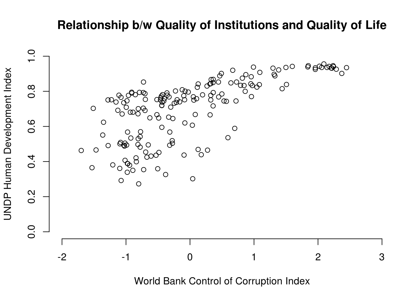
Sometimes people will report the correlation coefficient which is a measure of linear association and ranges from -1 to +1. Where -1 means perfect negative relation, 0 means no relation and +1 means perfect positive relation. The correlation coefficient is commonly used as as summary statistic. It’s diadvantage is that you cannot see the non-linear relations which can using a scatterplot.
We take the correlation coefficient like so:
cor(y = world.data$undp_hdi, x = world.data$wbgi_cce, use = "complete.obs")[1] 0.6821114| Argument | Description |
|---|---|
x |
The x variable that you want to correlate. |
y |
The y variable that you want to correlate. |
use |
How R should handle missing values. use="complete.obs" will use only those rows where neither x nor y is missing. |