6.2 Solutions
rm(list = ls())
setwd("~/PUBLG100")
6.2.1 Question 1
Using better model, where we included the square of GDP/capita, what is the effect of: a. an increase of GDP/capita from 5000 to 15000? b. an increase of GDP/capita from 25000 to 35000?
# load world data
a <- read.csv("QoG2012.csv")

# rename variables
names(a)[which(names(a)=="undp_hdi")] <- "human_development"
names(a)[which(names(a)=="wbgi_cce")] <- "institutions_quality"
names(a)[which(names(a)=="wdi_gdpc")] <- "gdp_capita"

# drop missings
a <- a[ !is.na(a$gdp_capita), ]
a <- a[ !is.na(a$human_development), ]
a <- a[ !is.na(a$institutions_quality), ]

# create factor again
a$former_col <- factor(a$former_col, labels = c("never colonies", "ex colonies"))

# re-run better modes
better.model <- lm(human_development ~ poly(gdp_capita, 2), data = a)
For a. we make two predictions. One, where gdp/capita is 5000 and one where it is 15000.
y_hat1 <- predict(better.model, newdata = data.frame(gdp_capita = 5000))
# predicted quality of life if gdp/capita is 5000
y_hat1
1
0.6443723 y_hat2 <- predict(better.model, newdata = data.frame(gdp_capita = 15000))
# predicted quality of life if gdp/capita is 15000
y_hat2 1
0.8272318 The effect of raising gdp/capita from 5000 to 15000 is the difference between our two predictions (called the first difference).
y_hat2 - y_hat1 1
0.1828595 The quality of life imporves by 0.18 according to our model when we raise gdp/capita from 5000 to 15000. Given that the human development index ranges from 0 - 1 (theoretical range), the effect is extremely large.
For b. we go through the same procedure.
y_hat1 <- predict(better.model, newdata = data.frame(gdp_capita = 25000))
y_hat2 <- predict(better.model, newdata = data.frame(gdp_capita = 35000))
y_hat2 - y_hat1
1
0.04116257 The quality of life improves by only 0.04 when we increase gdp/capita by 10 000 US$. Although, the increase in wealth was 10 000 in both scenarios, the effect is a lot more effective if the society is not already rich.
- You can see that the curve in our quadratic plot curves down when countries become very rich. Speculate whether that results make sense and what the reason for this might be.
6.2.2 Question 2
You can see that the curve in our quadratic plot curves down when countries become very rich. Speculate whether that results make sense and what the reason for this might be.
The downward curve does not make sense because it does not reflect a relationship that we actually observe in our data. The decline in life quality is due to the functional form of the square of gdp. It has to slope down at some point. We would not want to draw the conclusion that increasing wealth at some point leads to decline in the quality of life.
6.2.3 Question 3
Raise GDP/captia to the highest power using the poly() that significantly improves model fit. a. Does your new model solve the potentially artefical down-curve for rich countries? b. Does the new model improve upon the old model? c. Plot the new model.
To answer that question, we raise gdp/capita by one and compare model fit until adding another power does not improve model fit.
# power of 3
m.p3 <- lm(human_development ~ poly(gdp_capita, 3), data = a)
# compare cubic with quadratic using f test
anova(better.model, m.p3) # p < 0.05, so cubic is better
Analysis of Variance Table
Model 1: human_development ~ poly(gdp_capita, 2)
Model 2: human_development ~ poly(gdp_capita, 3)
Res.Df RSS Df Sum of Sq F Pr(>F)
1 169 1.8600
2 168 1.4414 1 0.41852 48.779 6.378e-11 ***
---
Signif. codes: 0 '***' 0.001 '**' 0.01 '*' 0.05 '.' 0.1 ' ' 1# power of 4
m.p4 <- lm(human_development ~ poly(gdp_capita, 4), data = a)
# compare models using f test
anova(m.p3, m.p4) # p < 0.05, so new model is betterAnalysis of Variance Table
Model 1: human_development ~ poly(gdp_capita, 3)
Model 2: human_development ~ poly(gdp_capita, 4)
Res.Df RSS Df Sum of Sq F Pr(>F)
1 168 1.4414
2 167 1.2653 1 0.17612 23.244 3.191e-06 ***
---
Signif. codes: 0 '***' 0.001 '**' 0.01 '*' 0.05 '.' 0.1 ' ' 1# power of 5
m.p5 <- lm(human_development ~ poly(gdp_capita, 5), data = a)
# compare models using f test
anova(m.p4, m.p5) # p < 0.05, so new model is betterAnalysis of Variance Table
Model 1: human_development ~ poly(gdp_capita, 4)
Model 2: human_development ~ poly(gdp_capita, 5)
Res.Df RSS Df Sum of Sq F Pr(>F)
1 167 1.2653
2 166 1.0193 1 0.24597 40.056 2.213e-09 ***
---
Signif. codes: 0 '***' 0.001 '**' 0.01 '*' 0.05 '.' 0.1 ' ' 1# power of 6
m.p6 <- lm(human_development ~ poly(gdp_capita, 6), data = a)
# compare models using f test
anova(m.p5, m.p6) # p < 0.05, so new model is betterAnalysis of Variance Table
Model 1: human_development ~ poly(gdp_capita, 5)
Model 2: human_development ~ poly(gdp_capita, 6)
Res.Df RSS Df Sum of Sq F Pr(>F)
1 166 1.01935
2 165 0.93283 1 0.086524 15.305 0.0001335 ***
---
Signif. codes: 0 '***' 0.001 '**' 0.01 '*' 0.05 '.' 0.1 ' ' 1# power of 7
m.p7 <- lm(human_development ~ poly(gdp_capita, 7), data = a)
# compare models using f test
anova(m.p6, m.p7) # p < 0.05, so new model is betterAnalysis of Variance Table
Model 1: human_development ~ poly(gdp_capita, 6)
Model 2: human_development ~ poly(gdp_capita, 7)
Res.Df RSS Df Sum of Sq F Pr(>F)
1 165 0.93283
2 164 0.87032 1 0.062509 11.779 0.0007582 ***
---
Signif. codes: 0 '***' 0.001 '**' 0.01 '*' 0.05 '.' 0.1 ' ' 1# power of 8
m.p8 <- lm(human_development ~ poly(gdp_capita, 8), data = a)
# compare models using f test
anova(m.p7, m.p8) # p > 0.05, so new model is worse!Analysis of Variance Table
Model 1: human_development ~ poly(gdp_capita, 7)
Model 2: human_development ~ poly(gdp_capita, 8)
Res.Df RSS Df Sum of Sq F Pr(>F)
1 164 0.87032
2 163 0.86650 1 0.0038174 0.7181 0.398The result is that raising gdp/captia to the power of seven provides the best model fit. We had to manually add powers of gdp to find the answer. For those of you are interested, there is a programmatic way to solve this problem quicker by writing a loop. We show you how to do so below. If you are interested, play around with this but you will not be required to be able to do this (we will not test you on this).
# the initial modle to compare to
comparison.model <- better.model
p <- 0.05 # setting a p-value
power <- 2 # the initial power

# loop until p is larger than 0.05
while(p <= 0.05){
  # raise the power by 1
  power <- power + 1
  # fit the new model with the power raised up by 1
  current.model <- lm(human_development ~ poly(gdp_capita, power), data = a)
  # run the f-test
  f <- anova(comparison.model, current.model)
  # extract p value
  p <- f$`Pr(>F)`[2]
  # comparison model becomes the current model if current model is better
  if (p <= 0.05) comparison.model <- current.model
}
screenreg(comparison.model)
====================================
                          Model 1
------------------------------------
(Intercept)                 0.70 ***
                           (0.01)
poly(gdp_capita, power)1    1.66 ***
                           (0.07)
poly(gdp_capita, power)2   -1.00 ***
                           (0.07)
poly(gdp_capita, power)3    0.65 ***
                           (0.07)
poly(gdp_capita, power)4   -0.42 ***
                           (0.07)
poly(gdp_capita, power)5    0.50 ***
                           (0.07)
poly(gdp_capita, power)6   -0.29 ***
                           (0.07)
poly(gdp_capita, power)7    0.25 ***
                           (0.07)
------------------------------------
R^2                         0.84
Adj. R^2                    0.84
Num. obs.                 172
RMSE                        0.07
====================================
*** p < 0.001, ** p < 0.01, * p < 0.05
a. Does your new model solve the potentially artefical down-curve for rich countries?
b. Does the new model improve upon the old model?
c. Plot the new model.We plot the polynomial to answer a) . To do so, we vary gdp/capita from its minimum to the maximum. This is the value of gdp values that we plot on the x axis. We use the predict() function to predict outcomes(\(\hat{Y}\)).
# our sequence of 100 GDP/capita values
gdp_seq <- seq(from = 226, to = 63686, length.out = 100)

# we set our covarite values (here we only have one covariate: GDP/captia)
x <- data.frame(gdp_capita = gdp_seq)

# we predict the outcome (human development index) for each of the 100 GDP levels
y_hat <- predict(m.p7, newdata = x)

# plot
plot(
  human_development ~ gdp_capita,
  data = a,
  pch = 16,
  frame.plot = FALSE,
  col = "grey",
  main = "Relationship between the quality of life and wealth",
  ylab = "Human development index",
  xlab = "GDP per capita"
  )

# plot polynomial
lines(x = gdp_seq, y = y_hat, lwd = 3, col = 1)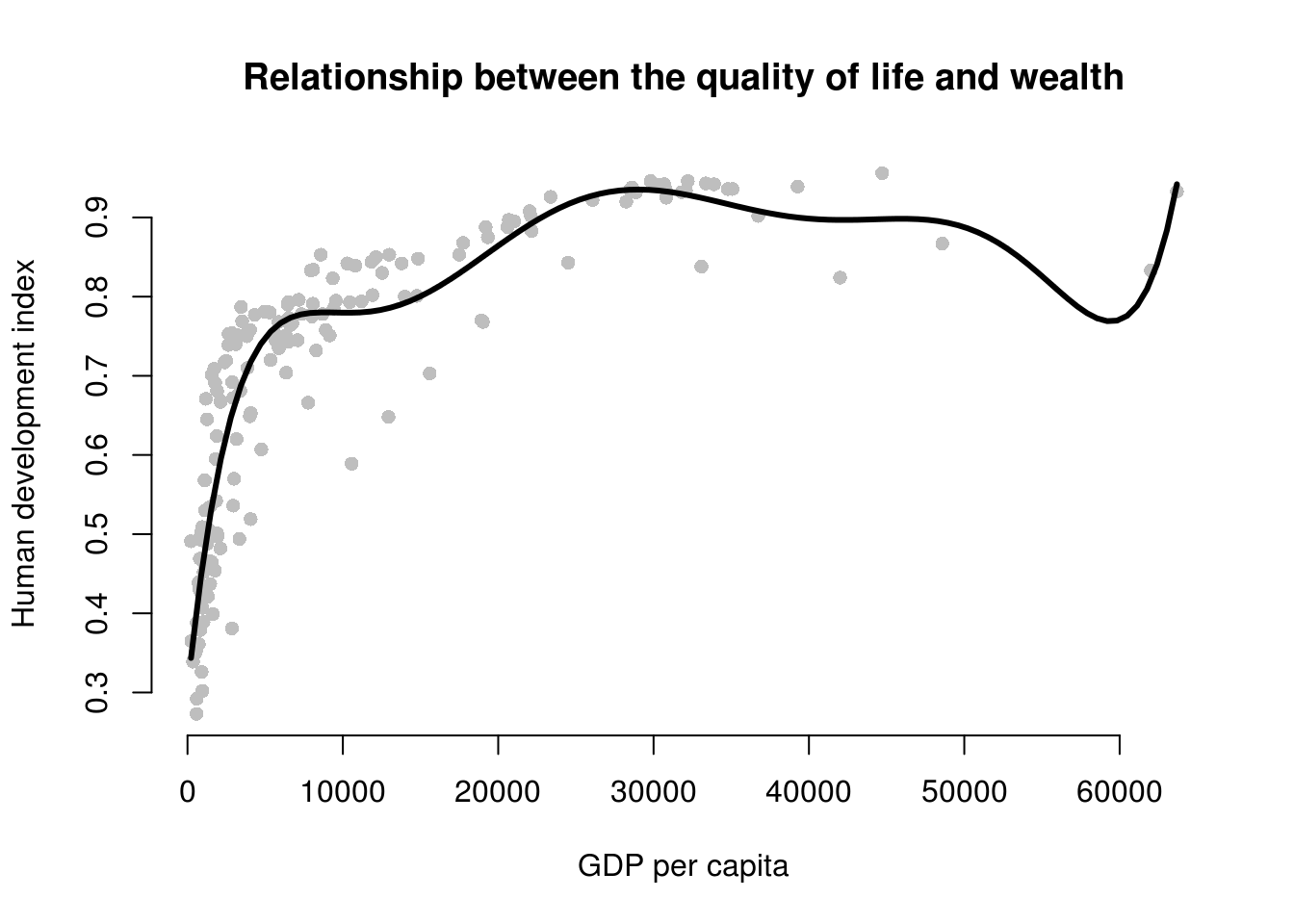
The model fit improves when we fit a 7th degree polynomial to the data. A seventh degree polynomial is very flexible, it can fit the points well. However, it is very important to remember that we have a sample of data. This sample is subject to sampling variability. That means our sample contains some ideosyncratic aspects that do not reflect the systematic pattern between GDP/captia and the human development index. We call the systematic pattern the “signal” and the random ideosyncratic bit “noise”.
Our 7th degree polynomial is too flexible. It fits the data in our sample too well. We almost certainly fit our model not just to the signal but also to the noise. We want to be parsimonious with our use of polynomials. Without advanced statistics, the general advise is to stay clear of higher degree polynomials. In published articles you often see a quadratic term. You may see a cubic term. Anything above is unusual.
6.2.4 Question 4
Estimate a model where wbgi_pse (political stability) is the response variable and h_j and former_col are the explanatory variables. Include an interaction between your explanatory variables. What is the marginal effect of: a. An independent judiciary when the country is a former colony? b. An independent judiciary when the country was not colonized? c. Does the interaction between h_j and former_col improve model fit?
m1 <- lm(wbgi_pse ~ h_j + former_col, data = a)
screenreg(m1)
=================================
                       Model 1
---------------------------------
(Intercept)             -0.32 *
                        (0.16)
h_j                      0.90 ***
                        (0.16)
former_colex colonies   -0.23
                        (0.16)
---------------------------------
R^2                      0.27
Adj. R^2                 0.26
Num. obs.              158
RMSE                     0.84
=================================
*** p < 0.001, ** p < 0.01, * p < 0.05
In this setting, an interaction does not make sense. We run a model on political stability (dependent variable). Our only two independent variables are the judiciary (h_j) and colonial past (former_col). With these two binary variables only, we have 4 possible combinations:
Judiciary = 0 and Ex colony = 0: \(\beta_0 = -0.32\) Judiciary = 1 and Ex colony = 0: \(\beta_0 + \beta_1 = 0.58\) Judiciary = 0 and Ex colony = 1: \(\beta_0 + \beta_2 = -0.55\) Judiciary = 1 and Ex colony = 1: \(\beta_0 + \beta_1 + \beta_2 = 0.35\)
In the model gives us information on all four possible combinations and we would not interact the dummy variables.
6.2.5 Question 5
Run a model on the human development index (hdi), interacting an independent judiciary (h_j) and control of corruption (corruption_control). What is the effect of control of corruption: a. In countries without an independent judiciary? b. When there is an independent judiciary? c. Illustrate your results. d. Does the interaction improve model fit?
m1 <- lm(human_development ~ institutions_quality * h_j, data = a)
screenreg(m1)
====================================
                          Model 1
------------------------------------
(Intercept)                 0.67 ***
                           (0.02)
institutions_quality        0.10 ***
                           (0.02)
h_j                         0.05 *
                           (0.03)
institutions_quality:h_j    0.01
                           (0.03)
------------------------------------
R^2                         0.48
Adj. R^2                    0.47
Num. obs.                 158
RMSE                        0.13
====================================
*** p < 0.001, ** p < 0.01, * p < 0.05- What is the effect of quality of institutions in countries without an independent judiciary?
The effect of institutions quality is \(\beta_1 = 0.10\).
- What is the effect of quality of institutions when there is an independent judiciary?
The effect of institutions quality is \(\beta_1 + \beta_3 = 0.10 + 0.01 = 0.11\).
- Illustrate your results.
# vary institutions quality
summary(a$institutions_quality)
Min. 1st Qu. Median Mean 3rd Qu. Max.
-1.69953 -0.81039 -0.28942 -0.01987 0.54041 2.44565 # sequence of quality of institutions
inst.qual <- seq(-1.7, 2.4, length.out = 100)
# set covariates when free judiciary is 0
x1 <- data.frame(institutions_quality = inst.qual, h_j = 0)
# set covariates when free judiciary is 1
x2 <- data.frame(institutions_quality = inst.qual, h_j = 1)
# predictions
y_hat1 <- predict(m1, newdata = x1)
y_hat2 <- predict(m1, newdata = x2)
# free judiciary
a$h_j <- factor(a$h_j, c(0, 1), c("controlled judiciary", "independent judiciary"))
# plot
plot(
human_development ~ institutions_quality,
data = a,
pch = 16,
frame.plot = FALSE,
col = h_j,
main = "Relationship between the quality of life and quality of institutions",
ylab = "Human development index",
xlab = "Quality of Institutions"
)
# add a legend
legend(
"bottomright", # position fo legend
legend = levels(a$h_j), # what to seperate by
col = a$former_col, # colors of legend labels
pch = 16, # dot type
lwd = 2, # line width in legend
bty = "n" # no box around the legend
)
# free judiciary = 0
lines(x = inst.qual, y = y_hat1, lwd = 3, col = 1)
# free judiciary = 1
lines(x = inst.qual, y = y_hat2, lwd = 3, col = 2)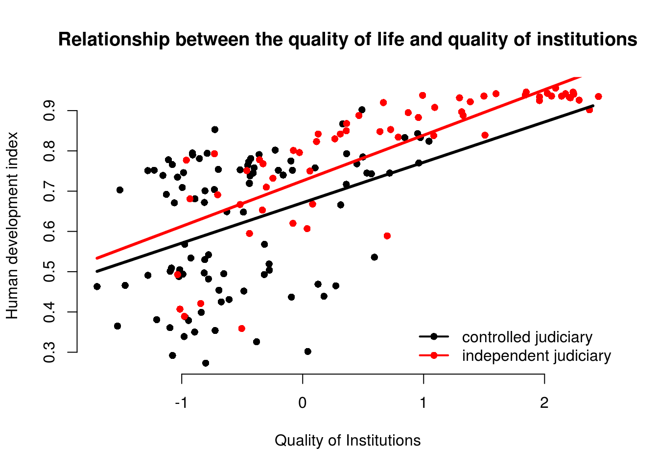
The effect of the quality of institutions does not seem to be conditional on whether a country has a controlled or an independent judiciary. The interaction term is insignificant and we can see that the slope of the lines is quite similar. We would not interpret the effect of the quality of institutions as conditional. It’s substantially similar in both groups.
m1 <- lm(human_development ~ institutions_quality * h_j, data = a)
screenreg(m1)
=========================================================
                                               Model 1
---------------------------------------------------------
(Intercept)                                      0.67 ***
                                                (0.02)
institutions_quality                             0.10 ***
                                                (0.02)
h_jindependent judiciary                         0.05 *
                                                (0.03)
institutions_quality:h_jindependent judiciary    0.01
                                                (0.03)
---------------------------------------------------------
R^2                                              0.48
Adj. R^2                                         0.47
Num. obs.                                      158
RMSE                                             0.13
=========================================================
*** p < 0.001, ** p < 0.01, * p < 0.05- Does the interaction improve model fit?
m_no_interaction <- lm(human_development ~ institutions_quality + h_j, data = a)
anova(m_no_interaction, m1)
Analysis of Variance Table
Model 1: human_development ~ institutions_quality + h_j
Model 2: human_development ~ institutions_quality * h_j
Res.Df RSS Df Sum of Sq F Pr(>F)
1 155 2.8102
2 154 2.8061 1 0.0041704 0.2289 0.633The f test confirms that the interaction model does not improve model quality. We fail to reject the null hypothesis that the interaction model does not explain the quality of life better.
6.2.6 Question 6
Clear your workspace and download the California Test Score Data used by Stock and Watson. a. Download ‘caschool.dta’ Dataset b. Draw a scatterplot between avginc and testscr variables. c. Run two regressions with testscr as the dependent variable. c.a. In the first model use avginc as the independent variable. c.b. In the second model use quadratic avginc as the independent variable. d. Test whether the quadratic model fits the data better.
- Load the dataset.
rm(list=ls())
library(foreign) # to load a stata file
a <- read.dta("caschool.dta")- Draw a scatterplot between
avgincandtestscrvariables.
plot(testscr ~ avginc, data = a,
     pch = 16,
     col = "darkgray",
     frame.plot = FALSE,
     xlab = "Average family income",
     ylab = "Student test scores")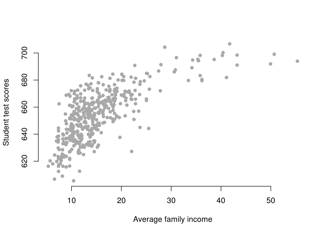
- Run two regressions with
testscras the dependent variable. c.a. In the first model useavgincas the independent variable. c.b. In the second model use quadraticavgincas the independent variable.
ca <- lm(testscr ~ avginc, data = a)
cb <- lm(testscr ~ poly(avginc,2), data = a)- Test whether the quadratic model fits the data better.
anova(ca, cb)Analysis of Variance Table
Model 1: testscr ~ avginc
Model 2: testscr ~ poly(avginc, 2)
Res.Df RSS Df Sum of Sq F Pr(>F)
1 418 74905
2 417 67510 1 7394.9 45.677 4.713e-11 ***
---
Signif. codes: 0 '***' 0.001 '**' 0.01 '*' 0.05 '.' 0.1 ' ' 1The quadratic model improves model fit. The p value is smaller than 0.05.
6.2.7 Question 7
- Load the
gunsdataset.- Pick a dependent variable that we did not use in class, that you want to explain. Why could explaining that variable be of interest (why should we care?)?
- Pick independent variables to include in the model. Argue why you include them.
- Control for potential confounders.
- Compare and discuss your best model and another model comprehensively.
rm(list=ls())
a <- read.csv("guns.csv")
names(a)
[1] "year" "vio" "mur" "rob" "incarc_rate"
[6] "pb1064" "pw1064" "pm1029" "pop" "avginc"
[11] "density" "stateid" "shall" Pick a dependent variable that we did not use in class, that you want to explain. Why could explaining that variable be of interest (why should we care?)? We pick violent crimes as a dependent variable
vio. Reducing violent crimes is a societal goal. At the same time, the means by which we can best achieve this goal is a subject of fierce debate.Pick independent variables to include in the model. Argue why you include them.
We test a deterrence argument. The more pople own guns, the more risky it is to comit a crime. Therefore, if everyone is armed to the teeth, crime rates will drop. Furthermore, a young person who comits a minor crime must immediately be sent to prison where the person sees real criminals. This will deter the young offender. In general, people will be deterred if prioson sentences are tough. We proxy tougher sentencing with the incarceration rate as a predictor variable to teest the argument that prison deters crime. We use the sahll laws predictor to test whether liberal gun laws lead to a reduction of violent crime.
m1 <- lm(mur ~ shall + incarc_rate , data = a)
screenreg(m1)
========================
             Model 1
------------------------
(Intercept)     1.71 ***
               (0.25)
shall          -3.68 ***
               (0.35)
incarc_rate     0.03 ***
               (0.00)
------------------------
R^2             0.55
Adj. R^2        0.55
Num. obs.    1173
RMSE            5.06
========================
*** p < 0.001, ** p < 0.01, * p < 0.05
In line with our original argument, laxer gun laws seem to reduce the violent crime rate. The incaceration rate, however, seems to increase violent crime.
- Control for potential confounders.
We control for average income. The argument is that crime is more prevalent in poorer areas. The variable could, therefore, confound the effect of the incaceration rate. We control for population density because urban areas are more affected by violent crime. We also control for the percentage of young men, who are the group in society who is most likely to comit violent crimes. As we discussed in the seminar there are potential confounders that vary across states but are constant over time. We, therefore, control for the states using fixed-effects. There are also potential confounders, as discussed in the seminar, that vary over time but are constant across states. Thus, we also control for time fixed-effects.
m2 <- lm(mur ~ shall + incarc_rate + pm1029 + avginc + density + factor(stateid) + factor(year), data = a)
screenreg(list(m1,m2),
          custom.model.names = c("Naive model", "State and Time Fixed Effects"),
          custom.coef.map = list(shall = "Shall", # list of variables we want displayed
                                 incarc_rate = "Icarceration Rate",
                                 pm1029 = "Percent Young Male",
                                 avginc = "Average Income",
                                 density = "Population Density"))
=============================================================
                    Naive model  State and Time Fixed Effects
-------------------------------------------------------------
Shall                 -3.68 ***     0.01
                      (0.35)       (0.32)
Icarceration Rate      0.03 ***     0.01 ***
                      (0.00)       (0.00)
Percent Young Male                  0.66 **
                                   (0.21)
Average Income                      0.99 ***
                                   (0.11)
Population Density                -10.65 ***
                                   (1.18)
-------------------------------------------------------------
R^2                    0.55         0.89
Adj. R^2               0.55         0.88
Num. obs.           1173         1173
RMSE                   5.06         2.59
=============================================================
*** p < 0.001, ** p < 0.01, * p < 0.05anova(m1, m2)Analysis of Variance Table
Model 1: mur ~ shall + incarc_rate
Model 2: mur ~ shall + incarc_rate + pm1029 + avginc + density + factor(stateid) +
factor(year)
Res.Df RSS Df Sum of Sq F Pr(>F)
1 1170 30011.8
2 1095 7338.8 75 22673 45.107 < 2.2e-16 ***
---
Signif. codes: 0 '***' 0.001 '**' 0.01 '*' 0.05 '.' 0.1 ' ' 1We compare the naive model with the one where we control for many confounders. Our small model is naive in the sense that there are almost certainly confounders that bias our estimates. We ran an F test which confirms that our bigger model is better at explaining the rate of violent crimes. Likewise, adjusted R^2 increases by a substantial amount. From the f test we can reject the hypothesis that our larger model is not better than the smaller and that our control variables really do not need to be in the model.
We argued that lax gun laws reduce the rate of violent crimes. The effect in the naive model was substantial and in line with our argument. After controlling for potential confounders, we found that effect is indistinguishable from zero. The most likely reason for the large change of the coefficient is omitted variable bias. We found no evidence for our argument that tougher sentencing reduces in crime in both models. The effect of the incaceration rate became smaller but reamains significant and positive. For a percentage point increase in the incarceration rate, the rate of violent crimes increases by 0.01 percentage points.
We are not interested in our control variables beyond the fact that we want to estimate unbiased effects of our deterrence variables. As expected, the larger the percentage of young males, the higher the rate of violent crime. Average income and population are significantlly related with crime but the direction of the correlation is unexpected.
Overall, we do not find evidence for our deterrence argument. The lax gun laws variable is unrelated to the rate of violent crimes. Tougher sentencing seems to be related to more violent crime, not less.
6.2.8 Question 6
Load the dataset from our lecture
a. Re-run the state fixed-effects model the lecture.
b. Run a state and time fixed-effects model.
c. Produce a regression table with both models next to each other but do not show us the dummy variables.
d. Interpret the models.rm(list=ls())
a <- read.csv("http://philippbroniecki.github.io/philippbroniecki.github.io/assets/data/resourcecurse.csv")- Re-run the state fixed-effects model the lecture.
summary(a) country countrycode year aid
Afghanistan: 12 AFG : 12 Min. :1996 Min. :-82.892
Albania : 12 ALB : 12 1st Qu.:2002 1st Qu.: 1.011
Argentina : 12 ARG : 12 Median :2004 Median : 2.611
Armenia : 12 ARM : 12 Mean :2004 Mean : 3.965
Australia : 12 AUS : 12 3rd Qu.:2007 3rd Qu.: 5.132
Azerbaijan : 12 AZE : 12 Max. :2010 Max. : 91.007
(Other) :804 (Other):804 NA's :38
oil gdp.capita institutions
.. :179 Min. : 58.08 Min. :-2.4797
0 :167 1st Qu.: 697.18 1st Qu.:-0.7741
0.000156118640282417: 1 Median : 2110.97 Median :-0.3653
0.000201585215662534: 1 Mean : 6473.18 Mean :-0.2333
0.000242650244292535: 1 3rd Qu.: 5706.16 3rd Qu.: 0.1476
0.00034466489898476 : 1 Max. :41904.21 Max. : 1.9833
(Other) :526 NA's :41
polity2 population mortality
Min. :-10.00 Min. :3.936e+05 Min. : 2.40
1st Qu.: -3.00 1st Qu.:4.427e+06 1st Qu.: 11.65
Median : 6.00 Median :1.050e+07 Median : 24.35
Mean : 3.37 Mean :6.116e+07 Mean : 35.71
3rd Qu.: 9.00 3rd Qu.:2.980e+07 3rd Qu.: 56.02
Max. : 10.00 Max. :1.338e+09 Max. :135.90
NA's :16 NA's :12 We look at a summary of the data first. The oil variable looks strange. We would have noticed that at the lasted when we run a model that includes oil. Because oil is a factor variable. It should be a numeric variable. The read.csv() function has converted oil to a factor variable. That only happens if not all entries are numeric but there are a few character entries in there as well. First of all, we look at the unique values of oil variable.
# umique values of oil variable
table(a$oil)
.. 0 0.000156118640282417
179 167 1
0.000201585215662534 0.000242650244292535 0.00034466489898476
1 1 1
0.000346878862548111 0.000467397247294325 0.000476450063796585
1 1 1
0.000507922025884573 0.000510052353010173 0.000536588343879004
1 1 1
0.00064049434964607 0.000678354261513085 0.000692243230603662
1 1 1
0.000714347794389084 0.000854805158781575 0.00101291415153668
1 1 1
0.00105614754722127 0.00108016933045609 0.00111410722261051
1 1 1
0.0014104248630006 0.00144698590145753 0.00147451590260641
1 1 1
0.00157224632629361 0.00162354239287375 0.00165400721913205
1 1 1
0.00181456436697681 0.0018328554755384 0.0019808182486859
1 1 1
0.00198739367968598 0.00200351779142715 0.00208010585915754
1 1 1
0.00224129073986938 0.00237079697904693 0.00237818897269424
1 1 1
0.00241217344914875 0.00256755526914228 0.00268078687927684
1 1 1
0.00270465094563035 0.00271197755055537 0.00321850963024146
1 1 1
0.00402851525723999 0.00414680727066109 0.00515219260492323
1 1 1
0.00516804316824336 0.00529760489806905 0.00531447974059541
1 1 1
0.00541663992631773 0.00663490576529441 0.00672136781408996
1 1 1
0.00680616633017334 0.00749860532629968 0.00837090101000204
1 1 1
0.00842108981916839 0.00994401148413807 0.010029386249079
1 1 1
0.0102723734983259 0.0112069685882833 0.0113136767829165
1 1 1
0.0117875054347387 0.0118600042980919 0.013216647219121
1 1 1
0.0138475364504411 0.0139146913687928 0.0141612105500983
1 1 1
0.014887674451979 0.0149194757811177 0.0151135044999419
1 1 1
0.0213394853640392 0.0213512343384014 0.0221781558781626
1 1 1
0.0229485039082304 0.0233819989312213 0.0292927454512843
1 1 1
0.029955399045163 0.030060273179477 0.030259497394368
1 1 1
0.0309442925615636 0.0344350102492647 0.0357493279267154
1 1 1
0.0365334700604582 0.0374734757724794 0.0385725575839389
1 1 1
0.0387453280736094 0.0394108857428631 0.0396181164827339
1 1 1
0.0405163709074161 0.0410649484359065 0.0428529693953669
1 1 1
0.0430820939359699 0.0442628767450202 0.0455229936142064
1 1 1
0.046279090384368 0.0465391823382496 0.0470894497418695
1 1 1
0.0484269350940646 0.050078413759947 0.0533495272835118
1 1 1
0.0552040073008234 0.0569677897554519 0.0604043085078517
1 1 1
0.070620017422454 0.0718602205879781 0.0738033935618876
1 1 1
0.0757435510857283 0.0768723690145049 0.0779203348430918
1 1 1
0.0795169528887435 0.0808831467593334 0.0823510022308636
1 1 1
0.083547205212876 0.0848269068654808 0.0881686275260491
1 1 1
0.0892276668050605 0.0899252685758644 0.0969599040303035
1 1 1
0.0995707424181358 0.101053891034491 0.101576260952683
1 1 1
0.104828075311191 0.107708544502072 0.110257335202643
1 1 1
0.110959164099508 0.113124668324475 0.12883800577866
1 1 1
0.128897087068449 0.129349905326733 0.136039483284248
1 1 1
0.138589047744828 0.1440830627703 0.14886025287306
1 1 1
0.158032625376662 0.158748407337589 0.159976303694402
1 1 1
0.167522503920329 0.173303738653033 0.173980267284975
1 1 1
0.176565770327093 0.176865891152218 0.183654871709533
1 1 1
0.19587660998538 0.196230306369697 0.208204968651365
1 1 1
0.21401612287026 0.216230033430904 0.219346833729918
1 1 1
0.222722618411046 0.224103101921053 0.232671497897705
1 1 1
0.233215266998557 0.242217917798885 0.275754158601241
1 1 1
0.276751659838538 0.280707735673487 0.289697409499122
1 1 1
0.314783513009109 0.318277246467813 0.320837731931226
1 1 1
0.321511717404299 0.323085987304958 0.331022517050861
1 1 1
0.339991320370978 0.35179116092985 0.381037592465392
1 1 1
0.381290629163125 0.396648202244149 0.435855390195356
1 1 1
0.445979673952247 0.447527590194189 0.48062761144049
1 1 1
0.483842492744298 0.488093256954193 0.50091744872931
1 1 1
0.512106699753118 0.523012659850713 0.540459698360425
1 1 1
0.548936494114521 0.56167521729512 0.575810525513394
1 1 1
0.590060667861136 0.601283560945899 0.629450410075873
1 1 1
0.646026951113171 0.650580487206376 0.654077767032296
1 1 1
0.654590548859491 0.660652737005066 0.682877501732518
1 1 1
0.689143851745227 0.691316553031657 0.702689829415199
1 1 1
0.705852320899757 0.707236836032986 0.711107155027003
1 1 1
0.73117377876177 0.751034891000837 0.752260918841924
1 1 1
0.754488464177443 0.759529531680359 0.76422793727721
1 1 1
0.771284811797749 0.775742875966664 0.780239074918585
1 1 1
0.810047753278887 0.81069421052457 0.840403021422887
1 1 1
0.842589086244412 0.850666770552889 0.863126744737264
1 1 1
0.864487980934801 0.865826640693169 0.867769128595759
1 1 1
0.869931894554092 0.8840895840028 0.900702525566347
1 1 1
0.913376338831758 0.914881888309388 0.917066961014983
1 1 1
0.930208323261257 0.94260421330197 0.954382573497724
1 1 1
0.955220973464334 0.955880919111228 0.957260243727537
1 1 1
0.957888357610237 0.976275696101909 0.984573853288986
1 1 1
0.989545049400784 1.00096831610427 1.02564133397501
1 1 1
1.03023504925458 1.03188110245328 1.04174123223649
1 1 1
1.05916254536436 1.06987433227152 1.07104433467616
1 1 1
1.082715030361 1.08479202503603 1.08896493881498
1 1 1
1.09214415213642 1.09973261064922 1.13165551460839
1 1 1
1.13253565773739 1.13926071071129 1.15369228103029
1 1 1
1.15556144363764 1.15652890029472 1.16767944088454
1 1 1
1.16924390598883 1.18483714779914 1.19249353490907
1 1 1
1.22841803163771 1.2288058225756 1.24025048662972
1 1 1
1.24033831038554 1.24046050123626 1.24813795159303
1 1 1
1.24901485264032 1.24944973652753 1.25517427918361
1 1 1
1.30299139993514 1.31141920158143 1.3251911326968
1 1 1
1.32707256357945 1.33719604006566 1.34263197537884
1 1 1
1.36569435512473 1.37976108871436 1.40064039506348
1 1 1
1.42290526720774 1.4238598798188 1.42471645736507
1 1 1
1.43764192891098 1.44653038165631 1.50084831301426
1 1 1
1.5303675714844 1.5344788299028 1.54228863770271
1 1 1
1.56433173620572 1.56668806058744 1.57495000359459
1 1 1
1.58581419729884 1.58636760794229 1.58961341652124
1 1 1
1.60570104751157 1.61016825526843 1.62156212975015
1 1 1
1.63082538834622 1.6328831293007 1.6485530368734
1 1 1
1.71055893622293 1.71082508502422 1.71645998554027
1 1 1
1.79400868906986 1.79689291029354 1.82481125050987
1 1 1
1.82969867556777 1.84305113982514 1.90137496549484
1 1 1
1.90911754741239 10.0593886168166 10.2428418950085
1 1 1
10.3026937486101 10.3259950259946 10.3384259490039
1 1 1
10.4449489442473 10.4634177203217 10.5380830508351
1 1 1
10.5637840781979 10.580118524004 10.7731181670379
1 1 1
10.9477000803789 11.1716268622481 11.1936755148867
1 1 1
11.2198345070262 11.6408410907144 11.7321743665156
1 1 1
11.8737186054061 12.1514196062491 12.7266167069131
1 1 1
12.7333530539327 12.9172681724516 13.5524144823992
1 1 1
14.0494620577367 14.2089472072279 14.2444774352273
1 1 1
14.254785575253 14.8098247089813 15.2013123124518
1 1 1
15.8392322501265 16.2271208310524 16.2454304430551
1 1 1
16.2731259891192 16.2823339520938 16.4744276481103
1 1 1
16.7436698058226 16.9629205620264 16.9674730799763
1 1 1
17.0651486442283 17.1088367806702 17.1357537404785
1 1 1
17.2718232052908 17.7260576267939 17.7332042882418
1 1 1
17.8081988042539 17.9766322342013 18.0453211444821
1 1 1
18.1727681625307 19.0798672454226 19.9717039157451
1 1 1
2.00497425496221 2.01119637165275 2.02032267506564
1 1 1
2.0288048746269 2.06583119882445 2.12950178914464
1 1 1
2.15386371725844 2.16648026144344 2.21845147774025
1 1 1
2.24402124173971 2.2747593173769 2.30390129429737
1 1 1
2.30972463405817 2.32187578211788 2.32827793675614
1 1 1
2.38613686958952 2.47326964350119 2.48246969629913
1 1 1
2.53735946168106 2.59229287955865 2.74465759052057
1 1 1
2.76900208334259 2.81864223962139 2.96285588869371
1 1 1
2.96985999680701 2.99643522892192 20.0258683461609
1 1 1
20.0658123341052 20.2060430728411 20.4263969631462
1 1 1
20.4321248059042 20.5170409360292 20.9345852809827
1 1 1
21.0236379113983 21.392575950889 21.8130023817884
1 1 1
21.8256685302275 21.8673426244217 22.4711356232666
1 1 1
23.0511305771239 23.2324340171604 23.2732773284622
1 1 1
23.464162456355 23.5261064331177 23.659822532068
1 1 1
23.8102650842349 23.8158812705224 24.0483162938322
1 1 1
24.0663695279098 24.3024087018727 24.3555149646988
1 1 1
24.3864669563398 24.7268276055521 24.8929356212503
1 1 1
24.9747439966191 26.5916193658903 26.7105154676532
1 1 1
26.8088921769981 27.054103568705 27.3496828422379
1 1 1
28.9404565790701 28.9975955934107 29.2152530659314
1 1 1
29.5940345495399 3.00830585302988 3.03550926238454
1 1 1
3.04402969252392 3.05812480123876 3.22104767201835
1 1 1
3.23773527471923 3.27009723385446 3.38610303079657
1 1 1
3.44183555056471 3.47113281393392 3.47170510064211
1 1 1
3.64640716604488 3.6755882659759 3.7297922301979
1 1 1
3.75417572014045 3.79594351086605 3.85324694115068
1 1 1
3.87421990814261 3.88139253211587 30.1711862967545
1 1 1
30.2405383504551 30.3636878691947 30.5114022839804
1 1 1
30.8396658813015 31.0524830035172 31.1393035633881
1 1 1
31.4193026847041 31.5413745241474 32.0242538095509
1 1 1
32.3468815510034 32.4214425339112 32.754473553782
1 1 1
33.0170733562321 33.4159983332954 34.5284952838343
1 1 1
34.6728813606149 35.6917502754748 35.8076218306893
1 1 1
36.2556616193899 36.6110564293678 36.7850749278227
1 1 1
37.7865701686021 38.2739126170236 38.6913837855008
1 1 1
39.084165250803 39.3395476875212 39.3400774626687
1 1 1
4.04881062162004 4.079037243848 4.22367432364308
1 1 1
4.22709763660241 4.23927380104914 4.36275706834052
1 1 1
4.54442720637317 4.55189096233028 4.57879777464852
1 1 1
4.70348755902276 4.71484282618384 4.85680182708014
1 1 1
40.2509661569359 40.6703496329503 40.8265315860986
1 1 1
41.2918089438098 41.6045738269634 41.7140640398282
1 1 1
47.8080181517174 5.04694670556947 5.17453961805956
1 1 1
5.3027223260555 5.31295293043136 5.35923418472799
1 1 1
5.39046415183157 5.41203357732249 5.57546886400765
1 1 1
5.59724184529389 5.66445325003662 5.68472922852651
1 1 1
5.80370723512351 5.88433816487573 5.89351077481128
1 1 1
5.9284868663226 50.4827932459081 51.0262067574282
1 1 1
51.0782619661917 51.3292247040161 54.9424794279018
1 1 1
6.33912146928285 6.37668888314792 6.48286125058122
1 1 1
6.57125041465221 6.73558521633143 6.91133982201089
1 1 1
6.97370193430111 6.98066497183166 61.5057894710875
1 1 1
63.2505843281866 64.3070502476404 7.08160587036391
1 1 1
7.13586909152281 7.23134750497845 7.25661318803335
1 1 1
7.66610270319159 7.86685787839947 7.99682000098976
1 1 1
8.12209577990561 8.2810515919459 8.43707371151447
1 1 1
9.05071290771452 9.16613892569635 9.20526881458493
1 1 1
9.39663185228582 9.52957483669086 9.67573725729883
1 1 1
9.7008001944997 9.77357323824612 9.8214073893474
1 1 1
9.85424433252832
1 The three dots are the way the World Banks codes missings by default. We have to convert them to NA. Firstly, we convert the factor variable to a string variable.
# convert factor variable to string
a$oil <- as.character(a$oil)
Now, we convert the variable from a string to numeric. R will convert all numbers it recognizes. It will not recognize the three dots and automatically turn them to NA.
# convert factor variable to string
a$oil <- as.numeric(a$oil)
Warning: NAs introduced by coercionsummary(a$oil) Min. 1st Qu. Median Mean 3rd Qu. Max. NA's
0.00000 0.00051 0.64603 5.68577 4.85680 64.30705 179 As we can see, the 179 observations that had the three dots are now NA’s.
We can now re-run the model from the lecture. Note that the country variable is already a factor variable in the data.
m1 <- lm(institutions ~ oil + aid + gdp.capita + polity2 + log(population) + country, data = a)- Run a state and time fixed-effects model.
m2 <- lm(institutions ~ oil + aid + gdp.capita + polity2 + log(population) + country + factor(year), data = a)- Produce a regression table with both models next to each other but do not show us the dummy variables.
screenreg(list(m1,m2),
          custom.model.names = c("State Fixed Effects", "State and Time Fixed Effects"),
          custom.coef.map = list(oil = "oil",
                                 aid = "aid",
                                 gdp.capita = "gdp/capita",
                                 polity2 = "polity score",
                                 `log(population)` = "log of population"))
====================================================================
                   State Fixed Effects  State and Time Fixed Effects
--------------------------------------------------------------------
oil                 -0.00                -0.00
                    (0.00)               (0.00)
aid                  0.00 *               0.00 *
                    (0.00)               (0.00)
gdp/capita           0.00                 0.00 **
                    (0.00)               (0.00)
polity score         0.01 ***             0.02 ***
                    (0.00)               (0.00)
log of population   -0.38 ***            -0.19 *
                    (0.06)               (0.08)
--------------------------------------------------------------------
R^2                  0.98                 0.98
Adj. R^2             0.98                 0.98
Num. obs.          672                  672
RMSE                 0.11                 0.11
====================================================================
*** p < 0.001, ** p < 0.01, * p < 0.05- Interpret the models.
Firstly, we look at the coefficient in a little more detail.
# we print the exact values of the first 6 coefficients
coef(m2)[1:6]
(Intercept) oil aid gdp.capita
2.339345e+00 -9.619829e-04 2.536486e-03 1.992969e-05
polity2 log(population)
1.656791e-02 -1.930962e-01 # we look at the range of the dependent variable
summary(a$institutions) Min. 1st Qu. Median Mean 3rd Qu. Max.
-2.4797 -0.7741 -0.3653 -0.2333 0.1476 1.9833 # so the range is roughly 4.5
# f test
anova(m1, m2)Analysis of Variance Table
Model 1: institutions ~ oil + aid + gdp.capita + polity2 + log(population) +
country
Model 2: institutions ~ oil + aid + gdp.capita + polity2 + log(population) +
country + factor(year)
Res.Df RSS Df Sum of Sq F Pr(>F)
1 609 7.8263
2 598 7.5656 11 0.26069 1.8732 0.04002 *
---
Signif. codes: 0 '***' 0.001 '**' 0.01 '*' 0.05 '.' 0.1 ' ' 1The variables oil and aid are oil rents as percentage of GDP and net international aid as percentage of GDP respectively. We discussed the rentier states theory in class. The hypotheses were that oil and aid should both reduce institutional quality (the dependent variable).
We do not find evidence for the theory. The effect of oil is insignificant in both models. Futhermore, aid seems to related to better quality institutions which would suggest that foreign aid does work.
The effect of aid is noticeable. When the percentage of foreign aid of gdp increases by a percentage point, the quality of institutions increases by 0.0025.
The magnitudes of the polity score increased. The effect of population almost halfed. These variables may have been confounded. Our model remains very stable. The F test suggests that, we improve model fit by controlling for time fixed effects as well.