6 Synthetic Control
Don’t have a good control unit to use in a difference-in-differences design? Don’t panic; just synthesise one. Synthetic control approaches allow for causal inferences based on similar assumptions to difference-in-differences, but are particularly well suited for situations in which the treatment occurs for a single unit. By providing a systematic way to choose comparison units, synthetic control is a good method for application to comparative case studies.
Synthetic control methods are a relatively new addition to the roster of causal inference techniques used in applied political science work. Because of this, there is no standard text-book treatment of these methods yet, at least that are we aware of. The best place to start reading therefore is this article by Abadie et al (2015) in the AJPS (you will recognise the Germany example from the lecture). The same authors also wrote a more detailed exposition of the method in this paper, which goes into more technical detail behind the estimation strategy. You can also consult this more recent paper by (the same) Abadie (2021)
For applications, the one we will focus on throughout the seminar is this paper by David Hope, who is at Kings College London. It may be inspirational to know that David started the project that resulted in this paper in a causal inference class very similar to the one you are currently taking! Another nice example of the synthetic control method is this paper by Benjamin Born and coauthors: in this study, the authors use synthetic control to estimate the costs of the Brexit vote to the UK economy. Finally, this very recent paper by Alrababa’h et al (2021) study the effect of football player Mohammed Salah’s coming to Liverpool F.C. on the incidence of hate crimes in the Liverpool area.
6.1 Seminar
The seminar this week is devoted to learning how to use the tidysynth package in R. This package has been developed to make it easier to implement synthetic control designs, though as you will see it does have a somewhat idiosyncratic coding style that is very step-by-step. You will need to install the package and load it as we have done in previous weeks, only this time by getting it directly from a github repository:
# install.packages("devtools")
# devtools::install_github("edunford/tidysynth") # Remember that you only need to install the package once
library(tidysynth)

# You may also need the ggplot2 package for further plot customisation (which we all love!)
library(ggplot2)
6.1.1 The Effect of Economic and Monetary Union on Spain’s Current Account Balance – Hope (2016)
In early 2008, about a decade after the Euro was first introduced, the European Commission published a document looking back at the currency’s short history and concluded that the European Economic and Monetary Union was a “resounding success”. By the end of 2009 Europe was at the beginning of a multiyear sovereign debt crisis, in which several countries – including a number of Eurozone members – were unable to repay or refinance their government debt or to bail out over-indebted banks. Although the causes of the Eurocrisis were many and varied, one aspect of the pre-crisis era that became particularly damaging after 2008 were the large and persistent current account deficits of many member states. Current account imbalances – which capture the inflows and outflows of both goods and services and investment income – were a marked feature of the post-EMU, pre-crisis era, with many countries in the Eurozone running persistent current account deficits (indicating that they were net borrowers from the rest of the world). Large current account deficits make economies more vulnerable to external economic shocks because of the risk of a sudden stop in capital used to finance government deficits.
David Hope investigates the extent to which the introduction of the Economic and Monetary Union in 1999 was responsible for the current account imbalances that emerged in the 2000s. Using the sythetic control method, Hope evaluates the causal effect of EMU on current account balances in 11 countries between 1980 and 2010. In this exercise, we will focus on just one country – Spain – and evaluate the causal effect of joining EMU on the Spanish current account balance. Of the \(J\) countries in the sample, therefore, \(j = 1\) is Spain, and \(j=2,...,16\) will represent the “donor” pool of countries. In this case, the donor pool consists of 15 OECD countries that did not join the EMU: Australia, Canada, Chile, Denmark, Hungary, Israel, Japan, Korea, Mexico, New Zealand, Poland, Sweden, Turkey, the UK and the US.
The hope_emu.csv file contains data on these 16 countries across the years 1980 to 2010. The data includes the following variables:
period– the year of observationcountry_ID– the country of observationcountry_no– a numeric country identifierCAB– current account balanceGDPPC_PPP– GDP per capita, purchasing power adjustedinvest– Total investment as a % of GDPgov_debt– Government debt as a % of GDPopenness– trade opennessdemand– domestic demand growthx_price– price level of exportsgov_deficit– Government primary balance as a % of GDPcredit– domestic credit to the private sector as a % of GDPGDP_gr– GDP growth %
Use the read.csv function to load the downloaded data into R now.
- Plot the trajectory of the Spanish current account balance over time (in red), compared to three other countries of your choice. Plot an additional dashed vertical line in 1999 to mark the introduction of the EMU. Would you be happy using any of them on their own as the control group?
# with ggplot2
library(ggplot2)
library(ggthemes)

# subset data to Spain, Japan, USA, and the UK
emu_sub <- emu[emu$country_ID %in% c("ESP","JPN","USA","GBR"),]

ggplot(emu_sub,aes(x=period,y=CAB,color=country_ID)) +
  geom_line() +
  geom_vline(xintercept = 1999, linetype="dashed") +
  scale_color_manual(values = c("red","blue","green","orange")) +
  ylab("Current Account Balance") + xlab("Year") +
  theme_clean() +
  theme(legend.title = element_blank(),
        legend.position = c(.15,.15))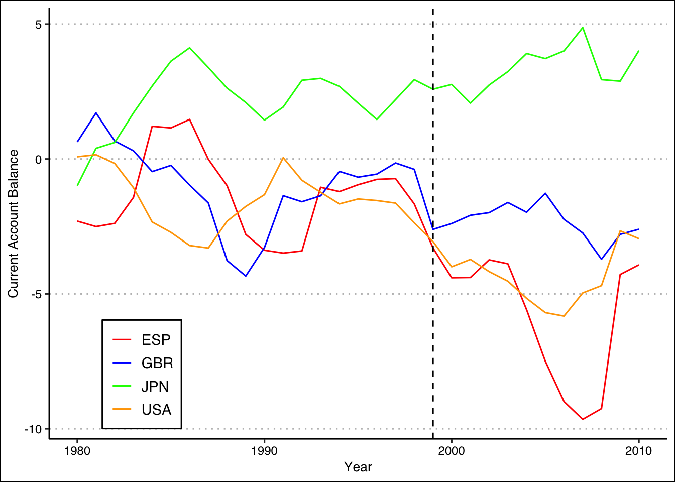
# With base-R
plot(x = emu[emu$country_ID == "ESP",]$period,
     y = emu[emu$country_ID == "ESP",]$CAB,
     type = "l",
     xlab = "Year",
     ylab = "Current Account Balance",
     col = "red",
     lwd = 3,
     ylim = range(emu$CAB)) # Because we are plotting multiple lines, we need to manually set the y-axis limits (here I am just using the range of the entire data)
lines(x = emu[emu$country_ID == "USA",]$period,
      y = emu[emu$country_ID == "USA",]$CAB,
      col = "orange")
lines(x = emu[emu$country_ID == "GBR",]$period,
      y = emu[emu$country_ID == "GBR",]$CAB,
      col = "blue")
lines(x = emu[emu$country_ID == "JPN",]$period,
      y = emu[emu$country_ID == "JPN",]$CAB,
      col = "darkgreen")
abline(v = 1999,
       lty = 3) # Lty specifies the line type (1 is solid, 2 dashed, 3 dotted, etc)
legend("topleft",
       legend = c("ESP","USA", "GBR", "JPN"),
       col = c("red", "orange", "blue", "darkgreen"),
       lty = 1,
lwd = 2) 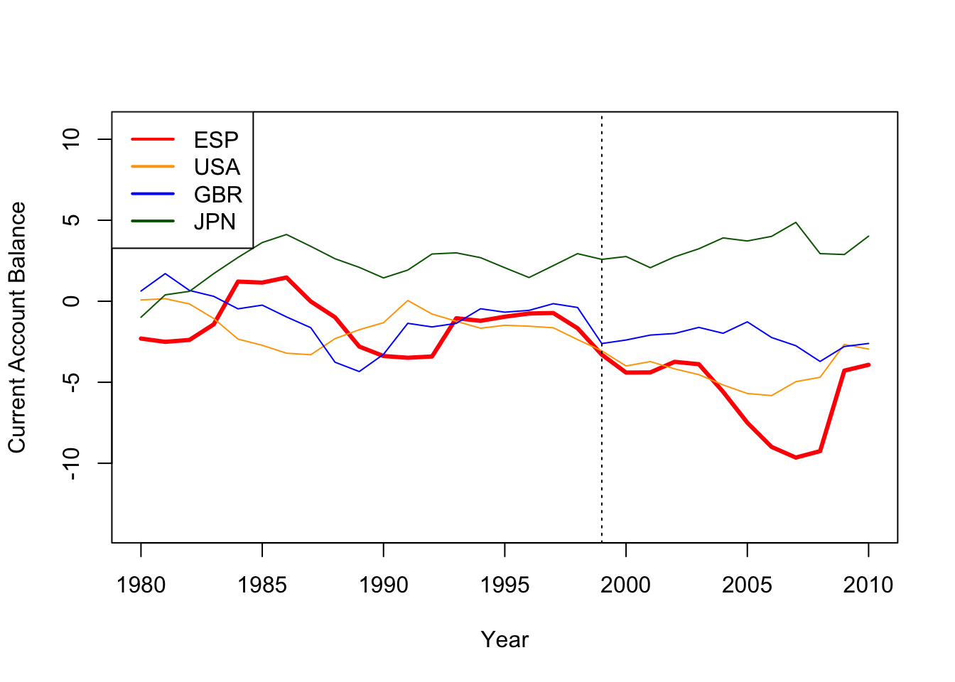
None of these individual countries is a perfect approximation to the pre-treatment trend for Spain, although the US and the UK lines are clearly closer than the Japanese line. The goal of the synthetic control analysis is to create a weighting scheme which, when applied to all countries in the donor pool, creates a closer match to the pre-intervention treated unit trend than any of the individual countries do alone.
- Preparing the synthetic control data:
Thetidysynthpackage takes data in a somewhat cumbersome way. You first need to ‘explain’ toRwhat the outcome variable, treatment and time identifier as well as the treated unit and start of treatment period are. This is done with the functionsynthetic_control(). Use this to prepare theemudata and store the result in a new object namedemu_synth. The main arguments you will need to use are summarised in the table below. Try on your own first, and then look at the solution below.
| Argument | Description |
|---|---|
data |
This is where we put the data.frame that we want to use for the analysis |
outcome |
The name of the dependent variable in the analysis (here, "CAB") |
unit |
The name of the variable that identifies each unit |
time |
The name of the variable that identifies each time period (must be numeric) |
i_unit |
The identifying value of the treatment unit (must correspond to the value for the treated unit in unit) |
i_time |
A vector indicating the start of the treatment period |
generate_placebos |
A logical value requesting that placebo versions of the data are created. Defaults to TRUE but, for now, set it to FALSE. |
Reveal answer
emu_synth <- synthetic_control(data = emu,
                               outcome = CAB,
                               unit = country_ID,
                               time = period,
                               i_unit = "ESP",
                               i_time = 1999,
                               generate_placebos = F)
The object you created (here we called it emu_synth) is a nested data set (where datasets are nested within cells of the the main dataset) with two rows. The first row contains the data for Spain and the second row contains the data from which the synthetic Spain will be constructed. You can have a look at the object by clicking on it in your environment and then clicking on the cells in the variable .outcome.
- Adding the predictor data:
In the next step, we need to specify which covariates should be considered in the calculation of the synthetic control weights for each donor unit. Remember, these covariates should be chosen according to whether they are predictive of the outcome. Further remember that the values need to be aggregated (usually averaged) across the entire pre-treatment period. The covariate are added with the functiongenerate_predictor()which takes the arguments listed below. Again, try this yourself, and then have a look at the solution.
| Argument | Description |
|---|---|
data |
The name of the object created with synthetic_control() (here, emu_synth) |
time_window |
The time window over which the data should be aggregated over. |
| … | Each variable to be added with its respective aggregation formula. For instance, to add the mean of variable GDPPC_PPP write GDPPC_PPP = mean(GDPPC_PPP, na.rm =T). Then add the next variable after a comma. |
Reveal answer
emu_synth <- generate_predictor(emu_synth, time_window = 1980:1998,
                                CAB = mean(CAB, na.rm=T),
                                GDPPC_PPP = mean(GDPPC_PPP, na.rm=T),
                                openness = mean(openness, na.rm=T),
                                demand = mean(demand, na.rm=T),
                                x_price = mean(x_price, na.rm=T),
                                GDP_gr = mean(GDP_gr, na.rm=T),
                                invest = mean(invest, na.rm=T),
                                gov_debt = mean(gov_debt, na.rm=T),
                                gov_deficit = mean(gov_deficit, na.rm=T),
                                credit = mean(credit, na.rm=T))
# note, the outcome variable should also be added as predictor!)
You will now see that a column was added to the object emu_synth called .predictors. If you click on each cell there, you will see that they are simply the aggregated values of each variables for Spain and each of the donor units, respectively.
- Calculating the synthetic control weights:
With the data now prepared and ready, the weights for each donor unit can be estimated. This is done withgenerate_weights(). There are a number of details of the estimation that can be fine tuned but we will simply use the defaults. The only arguments you will need are listed below. Note: It can take a few minutes for this function to run, so be patient!
| Argument | Description |
|---|---|
data |
The name of the object created with synthetic_control() and with the predictors added with generate_predictors() (here, emu_synth) |
optimization_window |
The time window of the pre-treatment period to be used in the optimization task. Here we will use the entire pre-treatment period. |
Reveal answer
This should now have added three new columns to the emu_synth object: .unit_weights contains what? the unit weights! We referred to these with the letter \(w\) in the lecture. .predictor_weights are the weights \(v\) for each variable. There is also another column called .loss which you can ignore here.
- Calculating the synthetic control:
Now, we are finally ready to create the synthetic control unit (i.e. multiplying the outcomes of the donor units for each time period by their estimated weight and summing them up). This is done simply by runninggenerate_control()on the object you created with the steps above.
This adds the final column we need, called .synthetic_control, which contains a data frame of the actual, observed, outcomes and the ‘sytnthetic’ outcomes for each time period. You can also extract that table directly with grab_synthetic_control(), although looking at many numbers like this is not very telling. Therefore, it is better to plot the synthetic control results, which we are doing in the next question.
## # A tibble: 6 × 3
##   time_unit real_y synth_y
##       <int>  <dbl>   <dbl>
## 1      1980  -2.30  -1.62
## 2      1981  -2.50  -1.55
## 3      1982  -2.39  -1.18
## 4      1983  -1.42   0.188
## 5      1984   1.21  -0.378
## 6      1985   1.15  -0.562
- Plotting the results:
Use tidysynth’splot_trends()andplot_differences()functions on theemu_synthobject to produce plots which compare Spain’s actual current account balance trend to that of the synthetic Spain you have just created. Interpret these plots. What do they suggest about the effect of the introduction of EMU on the Spanish current account balance? Hint: These functions create plots in the style ofggplot2so can be further customised as anyggplotwith+.
# absolute values
plot_trends(emu_synth) +
  labs(x="Year", y = "Current Account Balance (CAB)",subtitle = "Spain")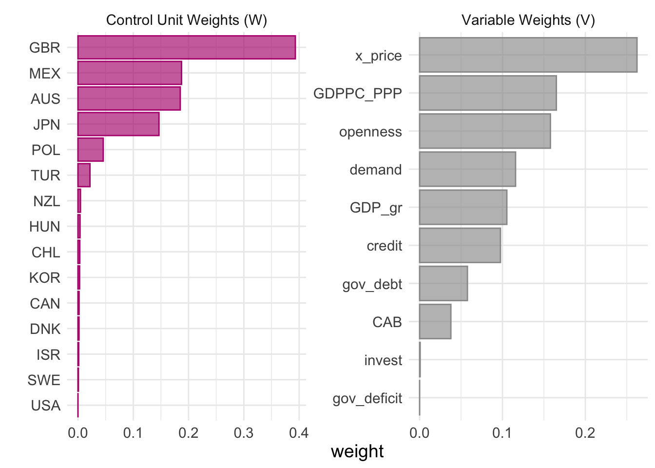
# difference between values
plot_differences(emu_synth) +
  labs(x="Year", y = "Current Account Balance (CAB) Difference",subtitle = "Spain")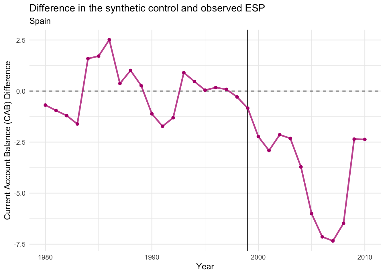
The synthetic version of Spain provides a reasonably good approximation to the pre-treatment trend of Spain, as there are only small differences in the Current Account Balance between real Spain and synthetic Spain before 1999.
In addition, it is clear that the trajectory of Spain and its synthetic control diverge significantly after the EMU is introduced in 1999. In particular, the actual Spanish current account balance deteriorated much more than the current account balances of the synthetic control unit in the post-EMU period. This therefore provides some empirical support for the hypothesis that the introduction of the EMU caused the current account balances of Spain to deteriorate.
- Interpreting the synthetic control unit:
A crucial strength of the synthetic control approach is that it allows us to be very transparent about the comparisons we are making when making causal inferences. In particular, we know that the synthetic Spain that we created in question 2 is a weighted average of the 15 OECD non-EMU countries in our data.
- What are the top five countries contributing to synthetic Spain? You can use the function
grab_unit_weights()to extract the \(w\) weights.- Which variables contribute the most to the synthetic control? Is the synthetic control unit closer to the treated unit in terms of the covariates than the sample mean? You can use the function
grab_predictor_weights()to extract the \(v\) weights andgrab_balance_table()for a table of the predictor means for the treated, synthetic and donor units.
# a
## extract the country weights
w <- grab_unit_weights(emu_synth)

## keep only the top 5
w <- w[order(w$weight,decreasing = T)[1:5],]

## make a nice table with kableExtra
library(kableExtra)
kable(w, booktabs=T, digits = 3) | unit | weight |
|---|---|
| GBR | 0.393 |
| MEX | 0.187 |
| AUS | 0.185 |
| JPN | 0.147 |
| POL | 0.046 |
As the table shows, the main contributors to synthetic Spain are Great Britain, Mexico, Australia and Japan, with a smaller contribution from Poland.
# b

## extract the variable weights
v <- grab_predictor_weights(emu_synth)

## extract the covariate balance table
b <- grab_balance_table(emu_synth)

## combine the two into one table
predictors <- merge(v,b)
kable(predictors[order(predictors$weight,decreasing = T),],
      booktabs = T, digits = 3, row.names = F) %>%
column_spec(1:2, border_right = T)| variable | weight | ESP | synthetic_ESP | donor_sample |
|---|---|---|---|---|
| x_price | 0.262 | 0.592 | 0.592 | 0.575 |
| GDPPC_PPP | 0.165 | 14196.194 | 14258.894 | 13491.601 |
| openness | 0.158 | 0.341 | 0.348 | 0.421 |
| demand | 0.116 | 0.028 | 0.028 | 0.031 |
| GDP_gr | 0.105 | 2.647 | 2.743 | 3.197 |
| credit | 0.098 | 73.372 | 72.938 | 63.499 |
| gov_debt | 0.058 | 44.618 | 48.543 | 62.271 |
| CAB | 0.038 | -1.327 | -1.340 | -1.910 |
| invest | 0.001 | 22.605 | 23.546 | 23.947 |
| gov_deficit | 0.000 | -1.433 | 1.183 | 1.301 |
grab_predictor_weights() gives the weights assigned to each of the predictor variables in the model. As this table shows, the highest weight is assigned to the x_price variable, which suggests that the price level of exports is an important predictor for matching the pre-treatment trend of current account balances in Spain to those of other countries. GDP per capita, the degree of domestic demand growth, and the degree of trade openness are all important for this reason as well.
grab_balance_table() gives the mean of each of the predictor variables in the Treated unit (Spain), the Synthetic unit that is constructed by the synthetic control method, and for the entire sample. It is clear from the table that for all these variables, the synthetic unit is a much closer match for the treated unit than is the sample as a whole. This is, in fact, the whole point of synthetic control! It allows us to construct a control unit that is as similar as possible to our treatment unit.
tidysynth also has a convenient punction called plot_weights() which presents the unit weights \(w\) and predictor weights \(v\) in a graphical format, as you can see below.

- Estimating a placebo synthetic control treatment effect:
One way to check the validity of the synthetic control is to estimate “placebo” effects – i.e. effects for units that were not exposed to the treatment. In this question we will replicate the analysis above for Australia, which did not join EMU in 1999.
- In constructing synthetic Australia, we must exclude Spain – the actual treatment unit – from the analysis. Before you repeat the steps above for Australia, create a new data.frame that doesn’t include the Spanish observations. Hint: Here you will want to select all rows of the
emudata for which thecountry_IDvariable is not equal to"ESP".- Now repeat the steps above to estimate the synthetic control for Australia.
- What does the estimated treatment effect for Australia tell you about the validity of the design for estimating the treatment effect of the EMU on the Spanish current account balance?
- Compare the treatment effects from the Australian synthetic control analysis and the Spanish synthetic control analysis in terms of the pre- and post-treatment root mean square error values.
# b.
## Prepare the data for Australia
emu_synth_australia <- synthetic_control(data = emu_australia,
                                         outcome = CAB,
                                         unit = country_ID,
                                         time = period,
                                         i_unit = "AUS",
                                         i_time = 1999,
                                         generate_placebos = F)

emu_synth_australia <- generate_predictor(emu_synth_australia, time_window = 1980:1998,
                                          CAB = mean(CAB, na.rm=T),
                                          GDPPC_PPP = mean(GDPPC_PPP, na.rm=T),
                                          openness = mean(openness, na.rm=T),
                                          demand = mean(demand, na.rm=T),
                                          x_price = mean(x_price, na.rm=T),
                                          GDP_gr = mean(GDP_gr, na.rm=T),
                                          invest = mean(invest, na.rm=T),
                                          gov_debt = mean(gov_debt, na.rm=T),
                                          gov_deficit = mean(gov_deficit, na.rm=T),
                                          credit = mean(credit, na.rm=T))

## Estimate the new synthetic control
emu_synth_australia <- generate_weights(emu_synth_australia, optimization_window = 1980:1998) # the weights
emu_synth_australia <- generate_control(emu_synth_australia) # the SC

## Plot the results
plot_trends(emu_synth_australia)  +
  labs(x="Year", y = "Current Account Balance (CAB)",subtitle = "Australia")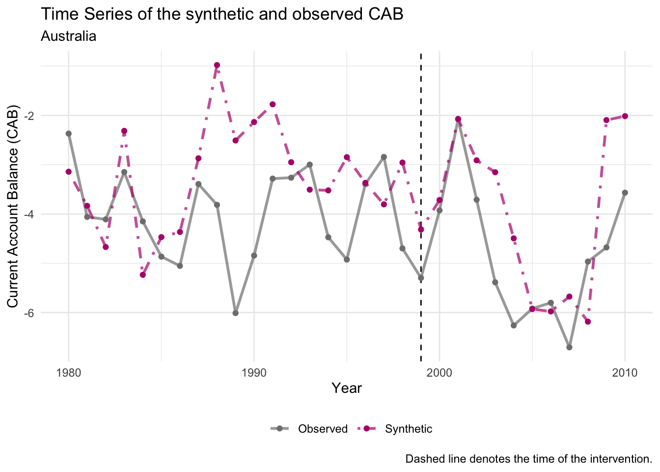
The placebo test here supports the inferences drawn from the main synthetic control analysis. There is clearly no effect of the introduction of EMU on the current account balance of Australia. Of course, full permutation inference would require re-estimating the synthetic control for every unit in the donor pool, not just Australia, and comparing the distribution of these placebo treatment effects to the treatment effect for Spain. In the homework, you will be asked to complete this analysis.
We can calculate the root mean squared prediction error for the pre-and post-intervention periods for both Australia and Spain. Recall that the the RMSE measures the size of the gap between the outcome of interest in each country and its synthetic counterpart. Large values of the ratio of the pre- and post-RMSEs provides evidence that the treatment effect is large. (We take the ratio of these measures because a large post-treatment RMSE is not itself sufficient evidence of a large treatment effect, because the synthetic control may be a poor approximation to the unit of interest. We account for the quality of the synthetic control unit by diving the post-treatment RMSE by the pre-treatment RMSE).
# Define function for calculating the RMSE
rmse <- function(x,y){
  sqrt(mean((x - y)^2))
}

# Define vector for pre/post-intervention subsetting
pre_intervention <- c(1980:2010) < 1999

## Spain
# extract outcome for synthetic spain
synthetic_spain <- grab_synthetic_control(emu_synth)$synth_y

# extract outcome for real spain
true_spain <- grab_synthetic_control(emu_synth)$real_y

# Calculate the RMSE for the pre-intervention period for spain
pre_rmse_spain <- rmse(x = true_spain[pre_intervention],
                       y = synthetic_spain[pre_intervention])

# Calculate the RMSE for the post-intervention period for spain
post_rmse_spain <- rmse(x = true_spain[!pre_intervention],
                        y = synthetic_spain[!pre_intervention])

# RMSE Ratio for spain
post_rmse_spain/pre_rmse_spain
## [1] 3.79421## Australia
# extract outcome for synthetic australia
synthetic_australia <- grab_synthetic_control(emu_synth_australia)$synth_y
# extract outcome for real australia
true_australia <- grab_synthetic_control(emu_synth_australia)$real_y
# Calculate the RMSE for the pre-intervention period for australia
pre_rmse_australia <- rmse(x = true_australia[pre_intervention],
y = synthetic_australia[pre_intervention])
# Calculate the RMSE for the post-intervention period for australia
post_rmse_australia <- rmse(x = true_australia[!pre_intervention],
y = synthetic_australia[!pre_intervention])
# RMSE Ratio for australia
post_rmse_australia/pre_rmse_australia## [1] 0.8859845The ratio of the RMSEs is much larger for Spain than for Australia, confirming the insight we took from the plots: the (null) placebo effect we estimated for Australia gives additional strength to our conclusion about the treatment effect we estimated for Spain.
6.1.2 The Effect of Economic and Monetary Union on Austria’s Current Account Balance – Hope (2016)
In the full paper linked to on the reading list (and above), Hope conducts the synthetic control analysis for several countries, not just for Spain. One particularly interesting case that he evaluates is Austria. Your task is to replicate the analysis we have just completed but this time using Austria, and not Spain, as the unit of interest. You will notice that the data provided for the seminar does not include any information about Austria, but you can download an additional, part-completed, dataset from the “Seminar data 2” link at the top of this page.
You will also notice that this additional data is missing one crucial variable: the outcome. Because you do not have any outcome variable here for the new treated unit, you will need to collect this yourself. In Hope’s paper, he suggests that the data on each country’s current account balance (measured as a % of GDP) can be found in the IMF World Economic Outlook Database, October 2015. You should be able to find the relevant data at this link. Your first task is to retrieve this information for Austria for the years 1980 to 2010, and to include that information in the Austria data set.
Once you have found the data and entered it into your downloaded csv file, you need to load both the Austria data and the main dataset from the seminar and combine them. To do so, you could use the rbind function that we introduced in last week’s seminar.
emu <- read.csv("data/hope_emu.csv")
austria <- read.csv("data/hope_emu_austria.csv")

austria$CAB <- c(...) # here you should enter the vector of CAB values

# Stack the data.frames on top of one another
emu_new <- rbind(emu, austria)
- Synthetic control for Austria:
You should now re-estimate the synthetic control method, this time using Austria as the unit of interest. Remember that you must ensure that you are not using Spain as a part of the donor pool. Then answer the following questions:
- Which 5 countries receive the highest weight as a part of synthetic Austria?
- Produce a plot which compares the current account balance of Austria to that of synthetic Austria. How does this compare to the equivalent plot of Spain?
- Retreive the vector of weights assigned to each of the variables used to construct synthetic Austria. Which variables contribute most to the synthetic control?
# Implement SCM for Austria
## prep data
emu_synth_austria <- synthetic_control(data = emu_new[emu_new$country_ID!="ESP",],
                                       outcome = CAB,
                                       unit = country_ID,
                                       time = period,
                                       i_unit = "AUT",
                                       i_time = 1999,
                                       generate_placebos = F)

## add predictors
emu_synth_austria <- generate_predictor(emu_synth_austria, time_window = 1980:1998,
                                        CAB = mean(CAB, na.rm=T),
                                        GDPPC_PPP = mean(GDPPC_PPP, na.rm=T),
                                        openness = mean(openness, na.rm=T),
                                        demand = mean(demand, na.rm=T),
                                        x_price = mean(x_price, na.rm=T),
                                        GDP_gr = mean(GDP_gr, na.rm=T),
                                        invest = mean(invest, na.rm=T),
                                        gov_debt = mean(gov_debt, na.rm=T),
                                        gov_deficit = mean(gov_deficit, na.rm=T),
                                        credit = mean(credit, na.rm=T))

## estimate weights
emu_synth_austria <- generate_weights(emu_synth_austria, optimization_window = 1980:1998)

## calculate synthetic control
emu_synth_austria <- generate_control(emu_synth_austria) # the SC
# a.
## extract the country weights
w <- grab_unit_weights(emu_synth_austria)
## keep only the top 5 and table
w <- w[order(w$weight,decreasing = T)[1:5],]
kable(w, booktabs=T, digits = 3) | unit | weight |
|---|---|
| JPN | 0.384 |
| POL | 0.205 |
| HUN | 0.198 |
| AUS | 0.189 |
| KOR | 0.021 |
- The main contributors to synthetic Austria are Japan, Australia, Poland, Hungary, and Korea.
# b.
plot_trends(emu_synth_austria) +
  labs(x="Year", y = "Current Account Balance (CAB)",subtitle = "Austria")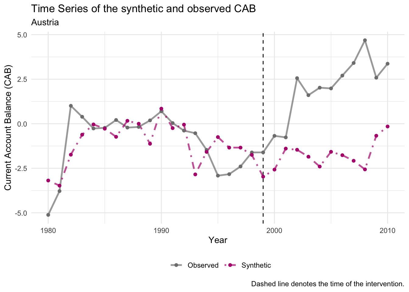
- In contrast to the Spanish case, the Austrian synthetic control demonstrates a worse current account balance than real Austria in the post-EMU period. These results imply that the EMU improved the current account position of Austria and worsened the current account position of Spain.
# c
v <- grab_predictor_weights(emu_synth_austria)
kable(v[order(v$weight, decreasing = T),], booktabs=T, digits = 3)| variable | weight |
|---|---|
| CAB | 0.306 |
| invest | 0.303 |
| GDP_gr | 0.227 |
| credit | 0.080 |
| gov_debt | 0.049 |
| demand | 0.028 |
| x_price | 0.006 |
| GDPPC_PPP | 0.000 |
| gov_deficit | 0.000 |
| openness | 0.000 |
- The largest two weights are assigned to the current account balance predictor, and the investment predictor, with much smaller weights placed on price level of exports, openness and GDP per capita (which seemed to matter more in the construction of synthetic Spain). Note that it is very common for the pre-treatment values of the dependent variable to be upweighted in the construction of the synthetic control, because the algorithm aims to produce a close fit between the synthetic unit and the treatment unit in the pre-treatment period.
- Permutation inference:
Conduct full permutation inference by estimating placebo treatment effects for all of the control units, and comparing them to the actual estimated effect for Spain (and/or Austria). This means calculating the MSPE ratios for each unit, and provide a plot summarising these statistics. This is wheretidysynthis really useful, meaning that rather than having to do the permutation inference by yourself by hand (i.e. calculate the placebo and the MSPE ratio for each donor unit like we did for Australia), you can simply re-do the steps from 1.2-1.5, only now you should specifygenerate_placebos = TRUEin the first step, as shown when clicking on ‘Reveal answer’. Then, you can have a look at the results of the results of the permutation inference by looking at the pre and post MSPE, their ratio and the coresponding p-values by runninggrab_significance(emu_synth_placebo). Or, if you prefer to display these graphically (which is generally easier to digest), you can useplot_placebos()as well asplot_mspe_ratio()to explore whether the results we (and the paper) find for Spain are likely to have occured by chance.
Reveal answer
## prepare data
emu_synth_placebo <- synthetic_control(data = emu,
                                       outcome = CAB,
                                       unit = country_ID,
                                       time = period,
                                       i_unit = "ESP",
                                       i_time = 1999,
                                       generate_placebos = T)
## add predictors
emu_synth_placebo <- generate_predictor(emu_synth_placebo, time_window = 1980:1998,
                                        CAB = mean(CAB, na.rm=T),
                                        GDPPC_PPP = mean(GDPPC_PPP, na.rm=T),
                                        openness = mean(openness, na.rm=T),
                                        demand = mean(demand, na.rm=T),
                                        x_price = mean(x_price, na.rm=T),
                                        GDP_gr = mean(GDP_gr, na.rm=T),
                                        invest = mean(invest, na.rm=T),
                                        gov_debt = mean(gov_debt, na.rm=T),
                                        gov_deficit = mean(gov_deficit, na.rm=T),
                                        credit = mean(credit, na.rm=T))
## estimate weights
emu_synth_placebo <- generate_weights(emu_synth_placebo, optimization_window = 1980:1998)
## calculate SC
emu_synth_placebo <- generate_control(emu_synth_placebo)## # A tibble: 16 × 8
## unit_name type pre_mspe post_mspe mspe_ratio rank fishers_exact_pvalue
## <chr> <chr> <dbl> <dbl> <dbl> <int> <dbl>
## 1 ESP Treated 1.31 21.0 16.0 1 0.0625
## 2 USA Donor 3.42 18.8 5.50 2 0.125
## 3 SWE Donor 5.42 13.3 2.46 3 0.188
## 4 JPN Donor 14.4 29.7 2.07 4 0.25
## 5 CAN Donor 3.36 6.72 2.00 5 0.312
## 6 HUN Donor 13.1 25.0 1.91 6 0.375
## 7 NZL Donor 4.94 6.48 1.31 7 0.438
## 8 TUR Donor 6.06 7.05 1.16 8 0.5
## 9 MEX Donor 6.32 6.29 0.995 9 0.562
## 10 GBR Donor 3.85 3.15 0.818 10 0.625
## 11 POL Donor 6.28 4.50 0.716 11 0.688
## 12 DNK Donor 6.17 3.20 0.518 12 0.75
## 13 AUS Donor 4.22 2.07 0.490 13 0.812
## 14 KOR Donor 25.6 4.94 0.193 14 0.875
## 15 CHL Donor 20.9 3.29 0.158 15 0.938
## 16 ISR Donor 14.9 1.65 0.111 16 1
## # ℹ 1 more variable: z_score <dbl>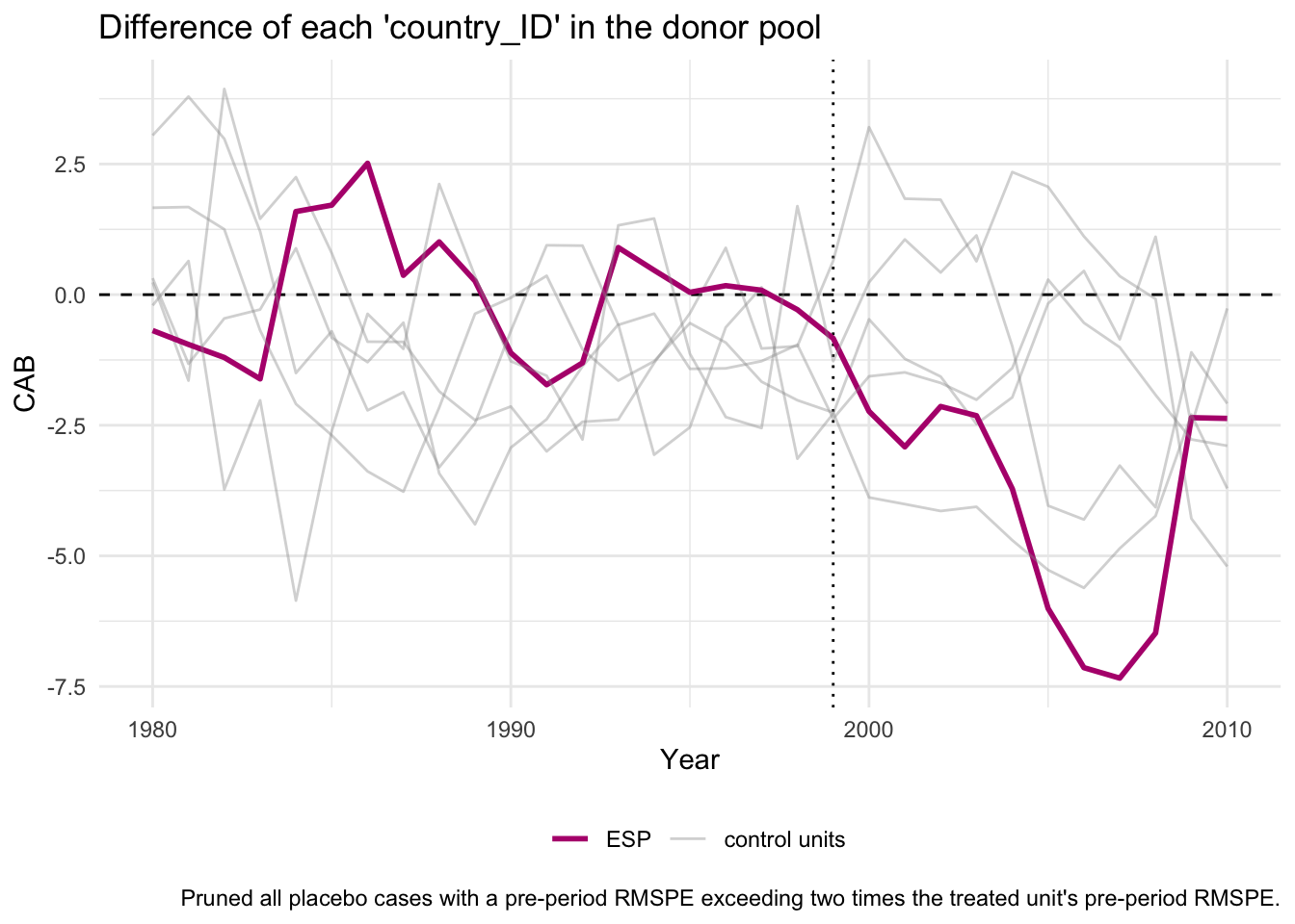
# MSPE ratios
plot_mspe_ratio(emu_synth_placebo) +
  annotate("label", x=2,y=12.5,
           label= expression("p ="~frac(1,16)~"=0.063"),
size=4) 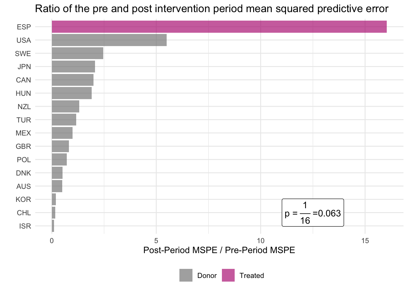
The MSPE ratio is higher when the effect of the EMU on the current account balance is larger. However, the measure also takes into account how well the synthetic control for each country can approximate the pre-EMU trend in current account balances. A large current account balance gap in the post-EMU period is not strong evidence of the EMU having a large effect if the synthetic control unit does not closely match the current account balance of the country of interest in the pre-EMU period. Put another way, a high post-EMU MSPE is not indicative of the EMU having a large effect on the current account balance when the pre-EMU MSPE is also large.
The results clearly show that this test statistic is far larger for Spain than for any other placebo countries in the donor pool. This implies that the results from the Spanish synthetic control analysis are very unlikely to have been driven by chance.
6.2 Quiz
- What is the main intuition behind the synthetic control method?
- To use post-treatment levels of the outcome variable for untreated units as a counterfactual for the post-treatment treated unit
- To use a weighted average of the post-treatment outcome variable for untreated units as counterfactual for the post-treatment treated unit
- To match the post-treatment outcome level of the treated unit to the post-treatment level of the closest untreated unit
- To randomly assign treatment to one and one unit only in our dataset, using the others as counterfactuals
- What is the estimand in a synthetic control design?
- An average treatment effect on the treated units (ATT) across the entire time period
- An average treatment effect on the treated units (ATT) for each time period
- An individual treatment effect (ITT) for the treated unit for each time period
- An individual treatment effect (ITT) for the treated unit across the entire time period
- How is the post-treatment synthetic control unit constructed?
- Remove all idiosyncrasies of treated or untreated units, and study exclusively within-unit variation
- Compare the difference between post-treatment and pre-treatment levels for the treated unit with the difference between post-treatment and pre-treatment levels for the control units, to remove all common shocks and idiosyncracies
- Assign more weight to untreated units that are closest to the treated one with respect to least predictive covariates and pre-treatment outcome levels. Compute the weighted average of Y at each time-point
- Assign more weight to untreated units that are closest to the treated one with respect to most predictive covariates and pre-treatment outcome levels. Compute the weighted average of Y at each time-point
- How can we make statistical inferences in a synthetic control (SC) design?
- Comparing a test statistic for the observed effect on a distribution of test statistics obtained by permuting the treatment assignment to each control unit in the donor pool and repeating the SC procedure
- By taking the ratio between the estimated effect size and the standard error associated with this measure and comparing this value over a t-student distribution
- We don’t need to draw statistical inferences because we are dealing with aggregate data, so we have perfect information and no uncertainty
- By clustering standard errors from the regression procedure by unit, to account for serial correlation
- How does the test statistic change in a SC design, with effect size and pre-treatment fit?
- It increases with larger post-treatment effects or with better pre-treatment fit
- It decreases with smaller post-treatment effects or with better pre-treatment fit
- It increases with smaller post-treatment effects or with worse pre-treatment fit
- It decreases with larger post-treatment effects or with worse pre-treatment fit