8 Instrumental Variables (II)
In this lecture we focus on the logic of instrumental variables in the context of observational studies. We will also discuss a number of applied examples that use an IV strategy, paying attention to how they work, and how they can go wrong.
“We describe our lives, our big choices, in narratives that blend conviction and luck, articulate plan and stumbling, seizing opportunity and being in the wrong place at the wrong time. We may be less than candid with ourselves and others in these narratives, but few would deny a role to luck.”
The quote above, found in Paul Rosenbaum’s excellent “Observation and Experiment” book (p. 258), nicely illustrates how many IV designs come to be. While we may not believe that the treatment that we care about has been randomly assigned, we hope to find an instrument that means that some part of the variation in that treatment can be thought of as random. This week we cover a number of examples of both good and (often) bad candidates for plausible instrumental variables, many of which are featured in greater detail in this week’s reading list.
In addition, some of the more mechanical detail on two-stage least-squares estimation that we covered in the lecture can be found on pages 173-186 of MHE, and there is a nice discussion of the exclusion restriction (and the difficulty of testing that assumption empirically) on pages 301-303 of the Morgan and Winship textbook. Finally, if you are looking for a lighter read – and don’t mind spending some money on another causal inference book – you can have a look at the entire chapter on IV in the Rosenbaum book mentioned above. It is notable because it features a rare combination of clear explanation, detailed examples, and funny anecdotes. Not something you say every day about an econometrics book.
Finally, as a way to further nourish a healthy skepticism about instrumental variables in observational settings, you can find some good points in a recent paper from Lal et al (2024).
8.1 Seminar
8.1.1 Do institutions cause growth? – Acemoglu, Johnson, and Robinson (2001)
The Acemoglu, Johnson, and Robinson (herein, AJR) paper entitled “The Colonial Origins of Comparative Development: An Empirical Investigation” is a classic example of instrumental variables estimation in the social sciences. AJR propose to study the relationship between a country’s institutions (measured with an index relating to the strength of property rights) and that country’s level of economic development (measured in modern day log GDP per capita) using settler mortality rates from the early 17th, 18th, and 19th centuries as an instrument.6
In terms of the notation we have been using, we can clarify the intuition behind AJR’s proposed strategy by using the following simplified notation:
- Instrument (\(Z_i \in \{1,0\}\)) – Settler mortality in the 17th, 18th and early 19th centuries (1 if settler mortality was high, 0 if settler mortality was low)
- Treatment (\(D_i\)) – Strong modern property institutions (1 if strong, 0 if weak)
- Outcome (\(Y_i\)) – Modern day wealth (GDP)
In the simplest terms, AJR use instrumental variables to estimate the effect of \(D_i\) on \(Y_i\) by instrumenting \(D_i\) with \(Z_i\). They find that strong modern property rights institutions causes higher GDP per capita.
Assumptions
- Name the four main assumptions underpinning instrumental variables as a strategy for identifying causal effects in the potential outcomes framework (i.e. name the assumptions needed to interpret the IV estimate as a LATE for compliers). Write out each assumption, and in your own words, interpret each assumption with regard to the specific setup of AJR’s study. Finally, discuss the plausibility of each assumption.
- Independence of the instrument – \(\{Y_{1i}, Y_{0i}, D_{1i}, D_{0i} \} \perp \!\!\! \perp Z_i\)
Independence in this case requires that settler mortality (\(Z_i\)) is independent of potential outcomes for \(Y_i\) and potential outcomes for treatment status \(D_i\) under \(Z_i\). That is, knowing the value of \(Z_i\) should not tell us anything about the potential log GDP per capita, nor the potential property rights institutions for each value of the instrument.
Is this plausible? First, note that we typically cannot assess this directly with data (in the same way that we cannot test independence directly in any other observational study). Theoretically, this assumption seems dubious in this example. Settler mortality is not assigned randomly – it is a function of among many factors, including: the disease environment, the latitude/longitude of an area, natural geography, agricultural feasibility, water access, and so on. Many of these factors could simultaneously correlate with both property rights institutions and log GDP per capita.
- Exclusion restriction – \(Y_i(Z_i = 1, D_i = d) = Y_i(Z_i = 0, D_i = d)\) for \(d \in \{1, 0\}\).
The exclusion restriction here requires that there is no effect of settler mortality on log GDP per capita other than through the effect of \(Z_i\) on \(D_i\). Is this plausible for AJR? Again, we cannot directly assess this empirically. From a theoretical perspective, however, we can imagine a number of potential ways in which \(Z_i\) could affect \(Y_i\) other than through its effect on \(D_i\). For instance, higher levels of settler mortality might have induced more conflict over resources, lowering log GDP per capita in the future. Or lower levels of settler mortality might have lead to more European settlements – as AJR argue – but the effect of the settlements on modern day GDP might have been transmitted through better established trade routes to European countries. There are many potentially plausible stories we could tell that would imply a violation of the exclusion restriction here, and would undermine the credibility of the IV estimates that AJR present.
- First-stage – \(0 < P(Z_i = 1) < 1\) & \(P(D_{1} = 1) \neq P(D_{0}=1)\)
The first stage assumption in the AJR case implies that settler mortality has a non-zero effect on modern day property rights institutions. That is, we should have a significant reduced form relationship between \(Z_i\) and \(D_i\). We can evaluate this assumption empirically, and will do below.
- Monotonicity – \(D_{1i} \geq D_{0i}\)
The monotonicity assumption is equivalent to stating that there should be no defiers in the population. In the AJR case, this implies that higher levels of settler mortality should always (weakly) push countries towards adopting more extractive (worse) institutions. This assumption does seem reasonable here, as it is hard to think of a (plausible) reason why some colonies would be defiers.
Replication
ajr.csv is a data set with observations for 64 countries, including information on the following variables:
GDP– log GDP per captia (adjusted for inflation, in 1995 US dollars)Exprop– average protection against expropriation risk (a continuous variable, and a proxy for institutions)Mort– settler mortality (measured as the number of individuals who died per 1000 people)logMort– log settler mortality (the logged version of theMortvariable)Latitude– the latitude of the countryLatitude2– the latitude of the country, squaredAfrica– dummy for AfricaAsia– dummy for AsiaNamer– dummy for North AmericaSamer– dummy for South AmericaNeo– dummy for Neo-Europe
- Estimate the effect of
ExproponGDPin two ways using regression. First, run a simple bivariate linear regression of those two variables, not including any other covariates. Second, run a multiple linear regression, including covariates forAfrica,Asia,NamerandSamer. Interpret the direction and statistical significance of the estimated coefficient forExpropfrom both models. Are these likely to be good estimates of the causal quantity of interest? Why, or why not?
| Dependent variable: | ||
| GDP | ||
| (1) | (2) | |
| Exprop | 0.522*** | 0.423*** |
| (0.061) | (0.058) | |
| Africa | -1.136*** | |
| (0.397) | ||
| Asia | -0.850** | |
| (0.405) | ||
| Namer | -0.223 | |
| (0.396) | ||
| Samer | -0.213 | |
| (0.402) | ||
| Constant | 4.661*** | 5.988*** |
| (0.409) | (0.612) | |
| Observations | 64 | 64 |
| R2 | 0.540 | 0.704 |
| Adjusted R2 | 0.532 | 0.678 |
| Residual Std. Error | 0.714 (df = 62) | 0.592 (df = 58) |
| F Statistic | 72.710*** (df = 1; 62) | 27.586*** (df = 5; 58) |
| Note: | p<0.1; p<0.05; p<0.01 | |
Using OLS, we find a positive association between average expropriation protections and log GDP per capita, significant at conventional levels. We should, of course, be cautious about interpreting these findings as causal as it seems very likely that there are omitted variables that simultaneously affect both levels of expropriation risk and levels of log GDP per capita.
- Use the same two regression approaches as in the question above, but this time estimate the effect of
logMortonGDP. Interpret the direction and statistical significance of the estimate of the causal effect. What does this “reduced form” model estimate? Under what conditions can we interpret this result as causal?
| Dependent variable: | ||
| GDP | ||
| (1) | (2) | |
| logMort | -0.566*** | -0.409*** |
| (0.078) | (0.098) | |
| Africa | -1.069* | |
| (0.536) | ||
| Asia | -0.900* | |
| (0.501) | ||
| Namer | -0.314 | |
| (0.498) | ||
| Samer | -0.305 | |
| (0.503) | ||
| Constant | 10.694*** | 10.663*** |
| (0.373) | (0.476) | |
| Observations | 64 | 64 |
| R2 | 0.462 | 0.562 |
| Adjusted R2 | 0.453 | 0.524 |
| Residual Std. Error | 0.772 (df = 62) | 0.720 (df = 58) |
| F Statistic | 53.245*** (df = 1; 62) | 14.886*** (df = 5; 58) |
| Note: | p<0.1; p<0.05; p<0.01 | |
The regression results suggest that higher levels of (logged) settler mortality are associated with lower levels of (logged) GDP per capita. The negative association between these two variables is significant at traditional levels. Because both the explanatory variable and the dependent variable are log transformed, the coefficients can be interpreted as elasticities: in the second model, a 1% increase in settler mortality is associated with a 0.05% percent decrease in GDP per capita on average, holding region constant.
The reduced form models here are estimators for the “intention-to-treat” effect (ITT) of settler mortality on log GDP per capita, under certain assumptions (I.e. we are estimating the total effect of \(Z_i\) on \(Y_i\)). The main assumption we require for this estimate to have a causal interpretation, of course, is that settler mortality is as good as randomly assigned, conditional on the covariates in the model (strictly speaking we also require the SUTVA assumption, which implies that there are no spillover effects of the instrument – this assumption is present in all of the methodological approaches we have studied on the course). It is also worth noting that, in this particular case, the reduced form relationship is not a particularly useful or interesting quantity with respect to answering the research question – we are not interested in the causal effect or settler mortality on GDP per capita!
- Estimate the first stage model for this problem. Remember, the first stage model should be a regression of \(D_i\) on \(Z_i\), potentially controlling for \(X_i\) (some covariates). Estimate these first stage models twice – once with and once without covariates (use the covariates that we used in the question above). Conduct an F-test for the first stage, for both models. Are you satisfied that the settler mortality instrument is sufficiently strong to serve as an instrument? Hint: you will need to use the
waldtestfunction in thelmtestpackage to estimate the F-tests. To estimate an F-test of a model without covariates, you just need to runwaldtest(model_name). This will produce the F-statistic comparing your model to a model only including the intercept – the “null” model. To estimate an F-test to compare two models, you just need to runwaldtest(model_1_name, model_2_name).
m1 <- lm(Exprop ~ Africa + Asia + Namer + Samer, ajr)
m2 <- lm(Exprop ~ logMort + Africa + Asia + Namer + Samer, ajr)

library(lmtest)
waldtest(m1,m2)
## Wald test
##
## Model 1: Exprop ~ Africa + Asia + Namer + Samer
## Model 2: Exprop ~ logMort + Africa + Asia + Namer + Samer
## Res.Df Df F Pr(>F)
## 1 59
## 2 58 1 6.3413 0.01458 *
## ---
## Signif. codes: 0 '***' 0.001 '**' 0.01 '*' 0.05 '.' 0.1 ' ' 1The F-test for weak instruments for the model with covariates produces an F-statistic of 6.3 in this example. The typical “rule of thumb” is that an F-statistic of under 10 suggests that the instrument may be too weak, and that the associated 2SLS coefficient on the instrumented treatment variable (i.e. the LATE) will be subject to bias. This result should therefore make us somewhat less confident about the causal effects we are about to estimate in the next question.
Note that if you calculate the F-test for the first stage model without covariates (see below), the F-statistic is much larger (23.34). This is because the F-statistic increases when the \(R^2\) of the full model (the model including the instrument) is much larger than the \(R^2\) of the restricted model (here, the restricted model is just the “null” model – i.e. a model with an intercept term but no regressors). When we only include the settler mortality instrument, but not the regional controls, the instrument explains a fairly large proportion of the variation in the treatment variable. However, when the controls are included, the instrument only contributes a small amount of additional explanatory power above and beyond the variation explained by the regional controls.
## Wald test
##
## Model 1: Exprop ~ logMort
## Model 2: Exprop ~ 1
##   Res.Df Df      F    Pr(>F)
## 1     62
## 2     63 -1 23.341 9.273e-06 ***
## ---
## Signif. codes:  0 '***' 0.001 '**' 0.01 '*' 0.05 '.' 0.1 ' ' 1
So, why don’t we just use the no-covariate model? Because remember that our assumption is that the settler mortality instrument is as good as random conditional on covariates! We therefore face a trade-off: If we were to exclude the regional dummies, our estimates will be subject to bias because our instrument will no longer satisfy the independence assumption. If we include those covariates, our instrument looks a little weak, which might also lead to bias. We will proceed by using both models to estimate the IV regression.
- Use the
ivregfunction in theAERpackage to estimate the local average treatment effect (LATE) for compliers ofExproponGDP, withlogMortused as the instrument. Again, do this twice: once with, and once without, covariates (remember, the same covariates need to be included in both the first- and second-stage models). Interpret the estimated LATE coefficient from both models. Additionally, retrieve the F-statistics for the first stage models estimated by theivregfunction (see the help file for the ivreg summary function (?summary.ivreg) for instructions of how to do this). Do they match the first-stage F-statistics that you calculated above?
library(AER)
iv_model_1 <- ivreg(formula = GDP ~ Exprop,
                    instruments = ~ logMort,
                    data = ajr)

iv_model_2 <- ivreg(formula = GDP ~ Exprop + Africa + Asia + Namer + Samer,
                    instruments = ~ logMort + Africa + Asia + Namer + Samer,
                    data = ajr)

texreg::screenreg(list(iv_model_1,iv_model_2))
##
## ================================
## Model 1 Model 2
## --------------------------------
## (Intercept) 2.04 * 1.51
## (1.00) (2.53)
## Exprop 0.92 *** 0.93 **
## (0.15) (0.28)
## Africa 0.34
## (0.98)
## Asia -0.06
## (0.75)
## Namer 0.86
## (0.83)
## Samer 0.81
## (0.82)
## --------------------------------
## R^2 0.22 0.31
## Adj. R^2 0.21 0.25
## Num. obs. 64 64
## ================================
## *** p < 0.001; ** p < 0.01; * p < 0.05# getting an `ivreg` model into a nice table is a bit cumbersome, as you see from the code below.
# This illustrate how there is not always a super convenient way to get your stuff into good tables...
# For the code below, I am using some functions and grammar of the tidyverse which
# may look very different from what you know. The usual disclaimer about the code
# complexity applies, so if this is too confusing, just ignore the following :)
library(tidyverse)
library(texreg)
library(kableExtra)
# This gives us the output from screenreg but in a matrix-object
modtab <- matrixreg(list(iv_model_1,iv_model_2))|>
as.data.frame() |>
`colnames<-`(c("term","Model 1","Model 2"))
modtab <- modtab[-1,]
# This code adds the F-test and Wu Hausman test below the model table
# I know this is horrible to look at. You are very welcome to just ignore it.
modtab2 <- rbind(summary(iv_model_1, diagnostics = T)$diagnostics[,3:4],
summary(iv_model_2, diagnostics = T)$diagnostics[,3:4]) |>
as.data.frame() |> drop_na() |>
mutate(term = rep(c("Weak instruments","Wu-Hausman"),2)) |>
rename("p.value"="p-value") |>
mutate(p.stars = ifelse(p.value<=0.05&p.value>0.01, "*",
ifelse(p.value<=0.01&p.value>0.001, "**",
ifelse(p.value<0.001, "***","")))) |>
mutate(across(where(is.numeric),~round(.,3))) |>
mutate(statistic = paste0(statistic,p.stars),
model = rep(c("Model 1","Model 2"),each=2)) |>
select(term,model,statistic) |>
pivot_wider(names_from = model, values_from = statistic) |>
mutate_all(as.character)
modtab <- modtab |> bind_rows(modtab2)
names(modtab)[1] <- " "
kable(modtab,booktabs =T) |>
kable_styling(full_width = F) |>
row_spec(12, hline_after = T) |>
add_header_above(c("","Log GDP per capita"=2))| Model 1 | Model 2 | |
|---|---|---|
| (Intercept) | 2.04 * | 1.51 |
| (1.00) | (2.53) | |
| Exprop | 0.92 *** | 0.93 ** |
| (0.15) | (0.28) | |
| Africa | 0.34 | |
| (0.98) | ||
| Asia | -0.06 | |
| (0.75) | ||
| Namer | 0.86 | |
| (0.83) | ||
| Samer | 0.81 | |
| (0.82) | ||
| R^2 | 0.22 | 0.31 |
| Adj. R^2 | 0.21 | 0.25 |
| Num. obs. | 64 | 64 |
| Weak instruments | 23.341*** | 6.341* |
| Wu-Hausman | 21.56*** | 9.804** |
If we are willing to assume the exclusion restriction and independence assumptions hold, and that the instrument is sufficiently strong to be free from bias, then the LATE estimates here suggest a substantively large and statistically significant causal effect of instutitions on GDP growth. Under these assumptions, a one-unit increase in the protection against expropriation risk measure causes an increase of .92 (no covariates) or .93 (with covariates) in log GDP.
The F-statistics from the ivreg function are identical to the ones calculated “manually” above, which means that we did that bit right!
8.1.2 Refugees and support for the far right – Dinas et. al. (2018)
In this section we will revisit the paper by Dinas et. al. which investigates the causal effect of the refugee crisis on support for the far right Golden Dawn party in Greece. In week 5’s seminar, we used a difference-in-differences approach to answer this question, but Dinas et. al. also use an IV approach in their paper, where they instrument for the number of refugees in a municipality using the distance of the municipality from the Turkish coast as an instrument.
The dinas_golden_dawn_iv.Rdata file (downloadable from the link at the top of the page) contains data on 96 Greek municipalities. In contrast to the data we studied in week 5, here we only have one observation per municipality (i.e. we are focusing only on cross-sectional variation, and ignoring the time dimension that we had last time). The muni data.frame contained within the new file therefore includes the following variables:
treatment– binary (1 if the observation is in the treatment group (a municipality that received many refugees).trarrprop– continuous (per capita number of refugees arriving in each municipality)gdvote_change– the outcome of interest. The change in the Golden Dawn’s share of the vote between January and September 2015. (Continuous)logdist– the logged distance of each municipality from the Turkish coast (originally measured in kilometers)
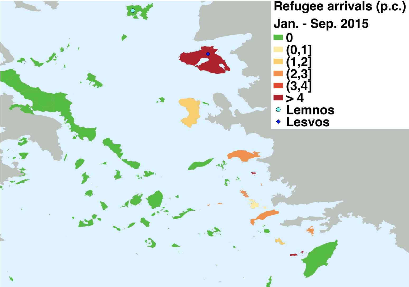
- First-stage relationship
The figure above shows graphically the idea behind the IV in this paper. It is clear that municipalities on islands that are situated closer to the Turkish coast were more likely to see inflows of refugees than municipalities on islands that were further away. In some sense, then, this plot is graphical evidence of the first-stage relationship that is required under the instrumental variables assumption.
Using the variablelogdist, calculate the first-stage effect ontreatment(the binary treatment indicator) andtrarrprop(the continuous treatment indicator). Conduct an F-test of these models against the null model (i.e. usingwaldtest). Are you satisfied with the results?
load("data/dinas_golden_dawn_iv.Rdata")

first_stage_binary <- lm(treatment ~ logdist, data = muni)
first_stage_continuous <- lm(trarrprop ~ logdist, data = muni)

waldtest(first_stage_binary)
## Wald test
##
## Model 1: treatment ~ logdist
## Model 2: treatment ~ 1
## Res.Df Df F Pr(>F)
## 1 93
## 2 94 -1 136.55 < 2.2e-16 ***
## ---
## Signif. codes: 0 '***' 0.001 '**' 0.01 '*' 0.05 '.' 0.1 ' ' 1## Wald test
##
## Model 1: trarrprop ~ logdist
## Model 2: trarrprop ~ 1
## Res.Df Df F Pr(>F)
## 1 92
## 2 93 -1 87.217 5.614e-15 ***
## ---
## Signif. codes: 0 '***' 0.001 '**' 0.01 '*' 0.05 '.' 0.1 ' ' 1In both cases, the F-statistic calculated for these models is very large (136 for the binary treatment, and 87 for the continuous treatment). We do not have to worry about weak instruments in this case.
- Estimating the LATE
Use instrumental variable regressions to estimate the effect of the refugee treatment (binary and continuous) on the change in vote share for the Golden Dawn, using thelogdistvariable as the instrument. What is the causal effect estimated from this model? How does it compare with the effects that we estimated using the difference-in-differences design in week 5?
The treatment effects here are very similar to those we estimated using the difference in differences design in week 5. In particular, the IV estimates suggest that the average treatment effect amongst complying municipalities is 2.08 (for the binary treatment), and 0.74 (for the continuous treatment). This implies that municipalities that received many refugees had about 2 percentage points higher support for the Golden Dawn, and that each additional refugee per captia causes an increase in the Golden Dawn’s vote share by about three-quarters of a percentage point. The equivalent coefficients for the diff-in-diff were 2.09 and 0.61. The fact that both estimation approaches – which are based on different identifying assumptions – give such similar results should strengthen our belief in these results.
- Exclusion Restriction
What is the exclusion restriction for this instrument? Are you persuaded that it holds? What test do the authors of this paper employ to try to strengthen their argument?
The exclusion restriction suggests that distance from the Turkish border has no effect on Golden Dawn vote share other than through the arrival of refugees. This seems a priori pretty reasonable, though it is possible that those islands have different pre-existing cultural or political perspectives that might affect support for the GD in different ways.
In order to strengthen their argument, Dinas et. al. use a particular feature of the Greek election law, in which registered but nonresident voters can cast their ballot in the town in which they they are registered, even if they do not live in the town they are registered in. The idea here is that the group of people who are registered in the treatment islands, but do not live there, are not actually exposed to the treatment, and so their vote shares should be no different to comparable people who are registered (but do not live) in the control islands. They use these groups of voters in a placebo test, which confirms that electoral support for the GD did not increase substantially among non-resident voters originating from treated islands between the two elections in 2015 when compared to non-resident voters of the control islands.
8.2 Quiz
- What is the purpose of an instrumental variable in an observational design?
- To overcome selection of units into/out of treatment
- To randomise treatment assignment
- To estimate a synthetic counterfactual for each unit in the sample
- To estimate unbiased standard errors for a causal effect
- What causal quantity is a 2SLS with multiple instruments estimating?
- An average treatment effect for units that are distributed around an artificial threshold
- An average treatment effect of each instrumental variables on the outcome variable, weighted by its relative strength
- An unweighted average of the LATEs computed with each instrument
- An average of the LATEs estimated with each instrument, weighted by the relative strength of their 1st stage
- What causal quantity is a 2SLS with covariates estimating?
- A weighted average of LATEs that are specific to each covariate-cell (combination of covariates)
- A weighted average treatment effect of each covariate on the outcome variable
- An individual treatment effect for each treated unit that complies with the instrument, conditional on covariates
- An average of the LATEs computed with each instrument, weighted by the relative strength of their 1st stage
- What causal quantity is a 2SLS with continuous treatment estimating?
- The average effect resulting from an infinitesimal change in treatment intensity
- A weighted average of the LATE only for units that comply with the treatment assignment
- A weighted average of the LATE for specific changes in treatment intensity induced by the instrument
- An unweighted average treatment effect after removing all idiosyncrasies between complying and non-complying units
- What assumption(s) of the IV design can be tested empirically, and how?
- The monotonicity, by checking the distribution of potential treatment condition under each treatment assignment condition
- The exclusion restriction assumption, by testing alternative paths through which the instrument affects the outcome
- The first-stage assumption, by performing an F-test on the restricted 1st stage model
- The independence assumption, by performing an F-test on the reduced-form model
The AJR paper has – at the most recent count – close to 20 thousand citations, and is heavily debated in a range of disciplines including economics, political science, and history. The questions here are highly stylized, and do not represent a fair characterization of the paper. I strongly encourage you to read the paper and surrounding debates carefully if you want to have a full understanding of this debate.↩︎