9 Regression Discontinuity Designs

A regression discontinuity design (RDD, for short) arises when the selection of a unit into a treatment group depends on a covariate score that creates some discontinuity in the probability of receiving the treatment. In this lecture we will consider both “sharp” and “fuzzy” RDDs.

Regression discontinuity designs are appropriate in cases where the probability that a unit is treated jumps at some specific value (\(c\)) of a running variable (\(X_i\)). The RDD is powered by the idea that jumps in the outcome (\(Y\)) that occur at the same value of the running variable can – under certain assumptions – be attributed to the causal effect of the treatment. The basic logic behind this is that we normally expect most outcomes to evolve smoothly, and so as long as we are able to model that smooth evolution to a sufficient degree of accuracy, we can calculate the difference in outcomes that occur at the cutoff and count that as the treatment effect.

There are good treatments (get it?) of the RDD in both the Mostly Harmless book, and the Mastering ’Metrics books, but it probably is easiest to gain intuition about these methods from seeing plenty of examples. The paper we covered during the lecture is this one by Andy Hall, which uses a very common RD setting – election results which lead to one type of candidate being elected rather than another type – but in an innovative way that speaks to some important debates in American Politics. For an example of population-threshold based RDDs, this paper by Andy Eggers is very nice. Eggers uses the fact that municipalities in France use one electoral system (Majoritarian) when they have a population of less than 3500 and another (PR) when they have more than 3500 people. Finally, this paper is really nice, where Ferwerda and Miller implement a geographic-RDD to investigate the causal effects of the Vichy regime in World War Two on the strength of the French resistance (you could also read this paper in which Kocher and Monteiro (2016) challenge the “as if random” interpretation of Ferwerda and Miller’s RDD setting.)

9.1 Seminar

9.1.1 Islamic Political Rule and Women’s Empowerment - Meyerson (2014)

Does Islamic political control affect women’s empowerment? Many countries have seen Islamic parties coming to power through democratic elections in recent years, and due to strong support among religious conservatives, constituencies with Islamic rule often tend to exhibit poor women’s rights. Does this reflect a causal relationship? Erik Meyerson examines this question by using data on a set of Turkish municipalities from 1994 when an Islamic party won multiple municipal mayor seats across the country. We will use this data and implement a regression discontinuity design to compare municipalities where this Islamic party barely won or lost elections.

This week we will need the rdrobust package for estimating regression discontinuity models and creating RD plots, and rddensity for density discontinuity tests. These packages implement modern, robust methods for RD analysis developed by Calonico, Cattaneo, Titiunik and co-authors. Install these packages now and load them into your environment.

# install.packages("rdrobust")
# install.packages("rddensity")
library(rdrobust)
library(rddensity)
library(ggplot2)
library(ggthemes)

You can load the data via:

islamic <- read.csv("data/islamic_women.csv")

The islamic_women.csv dataset includes the following variables:

margin – The margin of the Islamic party’s win or loss in the 1994 election (numbers greater than zero imply that the Islamic party won, and numbers less than zero imply that the Islamic party lost. 0 is an exact tie.)
school_men – the secondary school completion rate for men aged 15-20
school_women – the secondary school completion rate for women aged 15-20
log_pop – log of the municipality population in 1994
sex_ratio – sex ratio of the municipality in 1994
log_area – log of the municipality area in 1994

Estimating the LATE

Create a treatment variable within the data.frame islamic called islamic_win, that indicates whether or not the Islamic party won the 1994 election. In how many municipalities did the Islamic party win the election?

# Create the treatment variable
islamic$islamic_win <- as.numeric(islamic$margin > 0)

# Tabulate the treatment variable
table(islamic$islamic_win)

## 
##    0    1 
## 2332  328

The Islamic party won in 328 municipalities.

Calculate the difference in means in secondary school completion rates for women between regions where Islamic parties won and lost in 1994. Do you think this is a credible estimate of the causal effect of Islamic party control? Why or why not?

# Create the treatment variable
diff_in_means <- mean(islamic$school_women[islamic$islamic_win == 1], na.rm = T) -
  mean(islamic$school_women[islamic$islamic_win == 0], na.rm = T)

diff_in_means

## [1] -0.02577901

The difference in means is -0.0258. A naive interpretation of this would be that Islamic party control leads to lower female education rates. But this is not a very credible estimate of the causal effect, due to selection bias. The treated and untreated regions are likely to have very different potential outcomes; they are imbalanced. For example, it is likely that places that strongly support Islamic parties are less supportive of female education to begin with.

Before estimating the RDD, we need to select an appropriate bandwidth for the analysis. You can select the optimal bandwidth for this data using the rdbwselect function in the rdrobust package, which implements several data-driven bandwidth selection procedures including the so-called “MSE-optimal bandwidth”. After you have selected the optimal bandwidth, explain what the bandwidth means substantively in this case. Finally, using the bandwidth that you just calculated, create a new dataset that includes only those observations that fall within the optimal bandwidth of the running variable. Hint: You may need to read the help file (?rdbwselect) to see what the function requires.

bw_est <- rdbwselect(y = islamic$school_women, x = islamic$margin, c = 0)
summary(bw_est)

## Call: rdbwselect
## 
## Number of Obs.                 2630
## BW type                       mserd
## Kernel                   Triangular
## VCE method                       NN
## 
## Number of Obs.                 2315          315
## Order est. (p)                    1            1
## Order bias  (q)                   2            2
## Unique Obs.                    2313          315
## 
## =======================================================
##                   BW est. (h)    BW bias (b)
##             Left of c Right of c  Left of c Right of c
## =======================================================
##      mserd     0.172      0.172      0.286      0.286
## =======================================================

band <- bw_est$bws[1, 1] # extract the MSE-optimal bandwidth (h)
band

## [1] 0.1724268

This gives a bandwidth of approximately 0.17. This suggests that the optimal bias-variance trade-off is achieved for this specific RD analysis by only including municipalities where the vote share margin for the Islamic party was in the interval from approximately -0.17 to 0.17.

islamic_rdd <- islamic[abs(islamic$margin) < band, ]

Find the Local Average Treatment Effect of Islamic party control on women’s secondary school education at the threshold, using the dataset you created in the question above and a simple linear regression that includes the treatment and running variable. How credible do you think this result is?

# model
linear_rdd_model <- lm(school_women ~ margin + islamic_win, data = islamic_rdd)
# regression table
texreg::screenreg(linear_rdd_model)

## 
## =======================
##              Model 1   
## -----------------------
## (Intercept)    0.13 ***
##               (0.01)   
## margin        -0.22 ** 
##               (0.07)   
## islamic_win    0.03 ** 
##               (0.01)   
## -----------------------
## R^2            0.01    
## Adj. R^2       0.01    
## Num. obs.    795       
## =======================
## *** p < 0.001; ** p < 0.01; * p < 0.05

# Let's plot the relationship
## predicted values control
control <- data.frame(margin = seq(-round(band, 2), 0, .01), islamic_win = 0)
control$pred <- predict(linear_rdd_model, newdata = control)
## predicted values treated
treated <- data.frame(margin = seq(0, round(band, 2), .01), islamic_win = 1)
treated$pred <- predict(linear_rdd_model, newdata = treated)
## combine
pred <- rbind(control, treated)
pred$islamic_win <- as.factor(pred$islamic_win)

# Plot itself
ggplot(data = islamic_rdd, aes(x = margin, y = school_women)) +
  geom_point(alpha = .2) + # observed data
  geom_vline(xintercept = 0, linetype = "dotted") + # vertical line at cutoff
  geom_line(data = pred, aes(y = pred, color = islamic_win), linewidth = 1) + # regression line on either side of cutoff
  geom_segment(
    x = 0, 
    xend = 0,
    y = pred$pred[pred$margin == 0 & pred$islamic_win == 0],
    yend = pred$pred[pred$margin == 0 & pred$islamic_win == 1],
    linewidth = 1.5, color = "red") + # vertical line for LATE
  scale_y_continuous("Women Secondary School Completion Rate", limits = c(0, .6)) +
  scale_x_continuous("Islamic Party Election Margin", limits = c(-.2, .2), n.breaks = 5) +
  scale_colour_brewer("Islamic Party Win", palette = "Set2") +
  theme_clean() +
  lemon::coord_capped_cart(bottom = "both", left = "both") +
  theme(plot.background = element_rect(color = NA),
        panel.grid.major.y = element_blank(),
        legend.position = "bottom")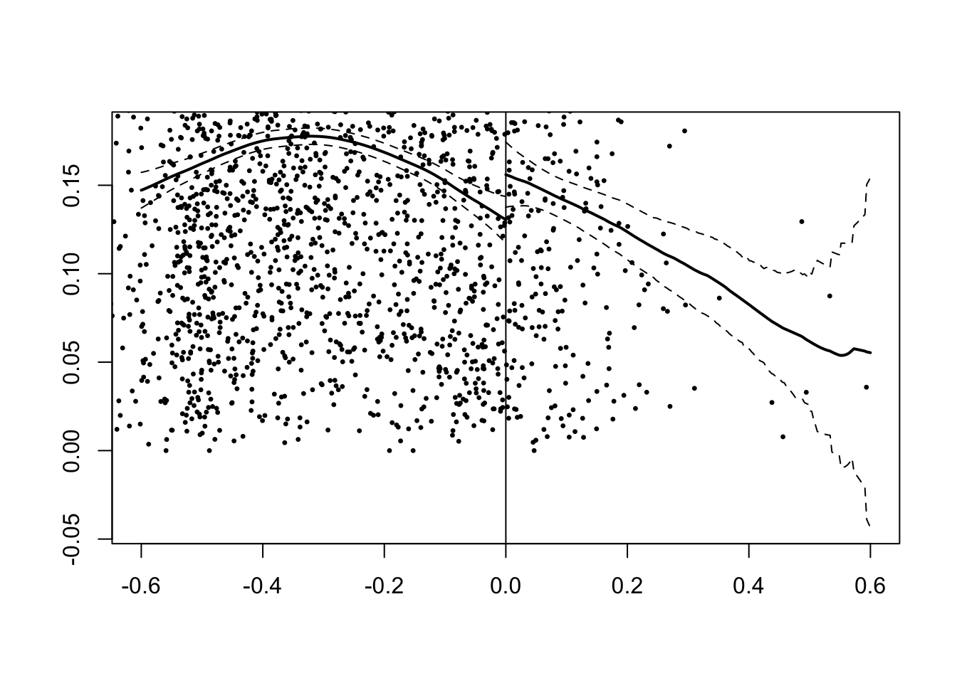

This gives a LATE estimate of 0.033 with a p value of 0.009, indicating that the effect is strongly statistically significant. This result may not be very credible because the model imposes that the relationship between female education and the running variable is linear and has the same slope on either side of the cutoff, since only a single coefficient on margin is estimated. These are strong assumptions. > 5. Use RD estimation to find the Local Average Treatment Effect of Islamic party control on women’s secondary school education at the threshold, using local polynomial regression estimated with the rdrobust function from the rdrobust package. Does the estimate differ from question 4?

The rdrobust function takes a number of arguments:

Argument	Description
`y`	The outcome variable.
`x`	The running variable (a.k.a. score or forcing variable).
`c`	The cutpoint, i.e. the value of the running variable at which the discontinuity is assumed to occur. Default is `c = 0`.
`h`	The bandwidth at which to estimate the RDD. If not specified, it is computed automatically using MSE-optimal bandwidth selection.
`all`	If `TRUE`, three estimation procedures are reported: conventional, bias-corrected, and robust. Default is `FALSE`, which only reports the robust procedure.

As always, you can read the help file for more information: ?rdrobust. Set all = TRUE so that you can compare the different estimation procedures in the output.

rd_est <- rdrobust(y = islamic$school_women, 
                   x = islamic$margin, 
                   c = 0, h = band, all = TRUE)
summary(rd_est)

## Sharp RD estimates using local polynomial regression.
## 
## Number of Obs.                 2630
## BW type                      Manual
## Kernel                   Triangular
## VCE method                       NN
## 
## Number of Obs.                 2315          315
## Eff. Number of Obs.             529          266
## Order est. (p)                    1            1
## Order bias  (q)                   2            2
## BW est. (h)                   0.172        0.172
## BW bias (b)                   0.172        0.172
## rho (h/b)                     1.000        1.000
## Unique Obs.                    2315          315
## 
## =======================================================================================
##         Method     Coef. Std. Err.         z     P>|z|      [ 95% C.I. ]       
## =======================================================================================
##   Conventional     0.030     0.014     2.116     0.034     [0.002 , 0.058]     
## Bias-Corrected     0.021     0.014     1.476     0.140    [-0.007 , 0.049]     
##         Robust     0.021     0.021     1.026     0.305    [-0.019 , 0.061]     
## =======================================================================================

Look first at the Conventional row of the output. Like the model in question 4, rdrobust uses local linear regression by default (p = 1). However, unlike question 4, it estimates separate regression lines on each side of the cutoff (rather than forcing the same slope) and applies kernel weights that give more influence to observations closer to the cutoff. The conventional LATE estimate is similar to the one from question 4: it gives us a LATE estimate of 0.030, with a p-value of 0.034, indicating that the effect is clearly significant at the 5% level.

The output also reports Bias-Corrected and Robust rows. These account for the bias inherent in local polynomial estimation at the MSE-optimal bandwidth – see the note below for details. For inference, you should use the Robust row, which pairs the bias-corrected point estimate with standard errors that account for the additional uncertainty from the bias correction step.

A note on bias correction and robust inference in rdrobust

When you look at the output from rdrobust, you will notice three rows of results: Conventional, Bias-corrected, and Robust. Understanding these requires some background on the bias-variance trade-off in RD estimation.

Why do we need bias correction?

Local polynomial RD estimators have two sources of error:

Variance, from sampling variability \(\rightarrow\) it decreases as the size of the bandwidth \(h\) increases, as we are including more data in the estimation.
Bias, from the fact that we are approximating a potentially curved regression function with a polynomial (e.g. linear, quadratic) \(\rightarrow\) the smaller the bandwidth, the fewer the observations the observations and the closer they are to the cutoff, so the better the polynomial approximation – and inversely. Therefore, the bias increases as \(h\) increases.

This gives rise to the classic bias-variance that is at the core of the bandwidth selection in modern RD methods. The MSE-optimal bandwidth aims to balance these two sources of error by minimzing the mean squared error (MSE), which is the sum of the variance and the squared bias. Yet, some bias remains at this optimal bandwidth. This bias is typically of the same order of magnitude as the standard deviation, because at the optimal bandwidth, the squared bias and the variance are ``balanced’’.

How does bias correction work?

The rdrobust package addresses this by explicitly estimating the bias using a higher-order polynomial. It can be shown that the bias of a local polynomial estimator of order \(p\) at the cutoff depends on the \((p+1)\)-th derivative of the regression function at the cutoff. For instance, if you fit a local linear regression (i.e., \(p=1\)), the bias depends on the second derivative of the regression function, that is, its curvature. The goal of bias correction is thus to estimate this \((p+1)\)-th derivative, which corresponds to the bias of the \(p\)-order local polynomial estimator, and to subtract this estimated bias from the original point estimate, to correct it.

Why do we need robust standard errors?

Estimating the bias and correcting the conventional point estimate introduces additional variability. Indeed, the bias-corrected point estimate is now a function of two estimated quantities, each of which has its own estimation error: the original point estimate and the estimated bias. Therefore, the variance of the bias-corrected point estimate is larger than that of the conventional point estimate, and we need to adjust the standard errors accordingly. Using the bias-corrected point estimate with the original standard errors would lead to undercoverage of confidence intervals and over-rejection of null hypotheses. The robust standard errors account for this additional variability, and they are the ones you should use for inference.

By the law of total variance, the variance of the bias-corrected estimator is equal to the variance of the original estimator plus the variance of the estimated bias, plus twice the covariance between the two estimators.
The robust standard errors are then obtained by taking the square root of this total variance.

Which results should I report?

For inference (hypothesis testing and confidence intervals), use the Robust row. This provides bias-corrected point estimates with standard errors that properly account for the uncertainty in both the main estimation and the bias correction. The robust confidence intervals have correct coverage properties at the MSE-optimal bandwidth.

For more details, see Calonico, Cattaneo, and Titiunik (2014), “Robust Nonparametric Confidence Intervals for Regression-Discontinuity Designs”, Econometrica.

Plot the relationship between the running variable and the outcome, with a line representing the local polynomial regression either side of the cutoff. Use your plot to explain why your results do or do not differ strongly between the linear RDD model you estimated in question 4 and the non-linear RDD model you estimated in question 5. Note: You do not need to produce this plot manually! You can use the rdplot function from the rdrobust package. For more options, look at the help file for ?rdplot.

rdplot(
  y = islamic$school_women, x = islamic$margin,
  c = 0,
  x.lim = c(-0.6, 0.6),
  title = "RD Plot: Islamic Party Win and Women's Education",
  x.label = "Islamic Party Election Margin",
  y.label = "Women Secondary School Completion Rate"
)

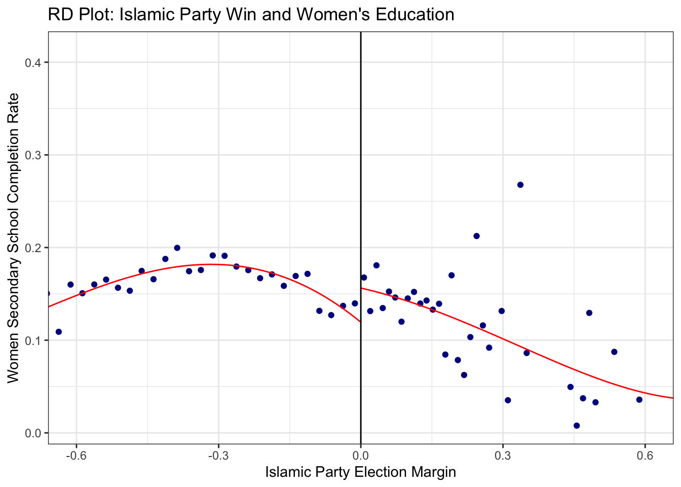
The plot indicates that the relationship between \(Y\) and \(\tilde{X}\) does appear to be approximately linear on either side of the cutoff. That explains why we received similar answers in both questions 4 and 5 above: linearity is a reasonable fit to the data here. That will not always be the case, though, and it is usually good practice to show that your results are insensitive to the functional form specification of the running variable.

Assessing the robustness of RD estimates

Note: In the robustness checks below, we report the bias-corrected estimates with robust standard errors (the Robust row from rdrobust output), as recommended for inference.

Perform placebo tests to check that the relationship between the running variable and outcome is not subject to discontinuities at values other than zero. To do this, re-estimate the RD, but varying the placebo cutoffs. Try values ranging from -0.1 to 0.1 incremented by 0.01. What do you conclude? You may also want to compare the ‘conventional’ and ‘robust’ estimates. Hint: Rather than writing the code for each separate cut-off, you can use a for loop. On each iteration of the for loop, estimate the RDD using that specific cutoff, and save the LATE estimates and the associated confidence intervals. Once the for loop is complete, we can simply plot the estimates and confidence intervals over the range of the cutoffs we specify. If you get stuck, click below to see some code to help you get started.

Reveal Code Hint

## Set the vector of cut-off points
cutpoint <- seq(from = -0.1, to = 0.1, by = 0.01)

## Setup some variables that can be used to store the estimates and confidence intervals
est <- rep(NA, length(cutpoint))
se <- rep(NA, length(cutpoint))

## Loop over the cut-offs
for (i in 1:length(cutpoint)) {
  ## Estimate the RD model with the appropriate cut-off here (using cutpoint[i])

  ## Extract the bias-corrected LATE coefficient from the model here (if rd_est is the
  ## estimated model, this can be found in rd_est$coef[3])
  ## and assign the estimated coefficient to the appropriate position in est

  ## Extract the robust standard error from the model here (if rd_est is the estimated
  ## model, this can be found in rd_est$se[3])
  ## and assign the estimated standard error to the appropriate position in se
}

## create a data.frame object with, as variables, cutpoint, est and se

## calculate the confidence intervals

# Doing this manually is tedious, as you can see:
# summary(rdrobust(y = islamic$school_women, x = islamic$margin, h = band, c = -0.1))
# summary(rdrobust(y = islamic$school_women, x = islamic$margin, h = band, c = -0.05))
# summary(rdrobust(y = islamic$school_women, x = islamic$margin, h = band, c = 0.05))
# summary(rdrobust(y = islamic$school_women, x = islamic$margin, h = band, c = 0.1))

# Let's use a loop instead!
## Set the vector of cut-off points
cut <- seq(from = -.1, to = 0.1, by = 0.01)

## Setup some variables that can be used to store the estimates and confidence intervals
est_c <- rep(NA, length(cut)) # conventional estimates
est_r <- rep(NA, length(cut)) # robust estimates
se_c <- rep(NA, length(cut)) # conventional standard errors
se_r <- rep(NA, length(cut)) # robust standard errors

for (i in 1:length(cut)) {
  ## Estimate the RD model with the appropriate cut-off
  rd_est_placebo <- rdrobust(
    y = islamic$school_women, x = islamic$margin,
    c = cut[i], h = band
  )
  
  est_c[i] <- rd_est_placebo$coef[1] # conventional estimate
  se_c[i] <- rd_est_placebo$se[1] # conventional standard error

  est_r[i] <- rd_est_placebo$coef[3] # bias-corrected estimate
  se_r[i] <- rd_est_placebo$se[3] # robust standard error
}

## create a data.frame object with, as variables, cut, est and se
out <- data.frame(est_c, se_c, est_r, se_r, cut)
out$truecut <- out$cut == 0

## calculate the confidence intervals
out$lo_c <- out$est_c - 1.96 * out$se_c
out$hi_c <- out$est_c + 1.96 * out$se_c
out$lo_r <- out$est_r - 1.96 * out$se_r
out$hi_r <- out$est_r + 1.96 * out$se_r

## plot
library(patchwork)
# conventional
p1 <- ggplot(out, aes(x = cut, y = est_c, color = truecut)) +
  geom_vline(xintercept = 0, linetype = "dotted") +
  geom_point() +
  geom_linerange(aes(ymin = lo_c, ymax = hi_c)) +
  geom_hline(yintercept = 0) +
  scale_x_continuous("Cut point", breaks = seq(from = -.1, to = 0.1, by = 0.05)) +
  scale_y_continuous("Estimate", breaks = seq(from = -.06, to = 0.04, by = 0.02)) +
  scale_color_manual(values = c("black", "red")) +
  labs(title = "Conventional Estimates") +
  theme_clean() +
  lemon::coord_capped_cart(bottom = "both", left = "both") +
  theme(
    plot.background = element_rect(color = NA),
    panel.grid.major.y = element_blank(),
    legend.position = "none",
    axis.ticks.length = unit(2, "mm"))

# robust
p2 <- ggplot(out, aes(x = cut, y = est_r, color = truecut)) +
  geom_vline(xintercept = 0, linetype = "dotted") +
  geom_point() +
  geom_linerange(aes(ymin = lo_r, ymax = hi_r)) +
  geom_hline(yintercept = 0) +
  scale_x_continuous("Cut point", breaks = seq(from = -.1, to = 0.1, by = 0.05)) +
  scale_y_continuous("Estimate", breaks = seq(from = -.06, to = 0.04, by = 0.02)) +
  scale_color_manual(values = c("black", "red")) +
  labs(title = "Robust Estimates") +
  theme_clean() +
  lemon::coord_capped_cart(bottom = "both", left = "both") +
  theme(
    plot.background = element_rect(color = NA),
    panel.grid.major.y = element_blank(),
    legend.position = "none",
    axis.ticks.length = unit(2, "mm"))

p1 / p2 + plot_annotation(title = "Placebo Tests: LATE Estimates at Different Cutoffs")

While there are no significant LATE estimates for the -0.05, 0.05 or 0.1 cutoffs, there is a significant (negative) treatment effect at the -0.1 cutoff. That is, the p-values for three of the cutoffs are large, while the p-value for the -0.1 cutoff is just 0.002. This is not hugely encouraging, as it suggests that there are significant discontinuities in the outcome variable for values of the running variable other than 0. This constitutes evidence against a true RD effect because it indicates that the discontinuity we measured at 0 could be only one of many discontinuities in the data. In other words, the effect at 0 could have arisen due to chance alone.

However, it is also noteworthy that the statistically significant effect estimated with cut-offs 0.1 and 0.09 is actually the other way around than the one at the ‘true’ cut-off zero. You can also see that in the plot below. Comparing this to the plot we got in the previous question, we see that those observations just below the (real) threshold (so where the islamic party narrowly lost) are the ones with surprisingly low share of women in school and are the ones pulling the estimated line downwards. One could surmise that candidates that won but narrowly against the islamic party got scared of their electoral success and over-compensated by trying to cater to a religious-conservative electorate which resulted in lower shares of women in school. Note that this is really just conjecture.

rdplot(
  y = islamic$school_women, x = islamic$margin, c = -0.1,
  x.lim = c(-0.6, 0.6),
  title = "RD Plot at Placebo Cutoff (-0.1)",
  x.label = "Islamic Party Election Margin",
  y.label = "Women Secondary School Completion Rate"
)

An alternative robustness check is to examine whether there are significant treatment effects for pre-treatment covariates that should not be affected by the treatment. Use the three pre-treatment covariates here – log_pop, sex_ratio, log_area – as outcome variables in new RD estimates. Do you find any significant effects of the treatment on these variables? Note: remember to set the h argument to be equal to the bandwidth that we selected in question 3 for all of these models.

rd_logpop <- rdrobust(y = islamic$log_pop, x = islamic$margin, h = band, c = 0)
rd_sexratio <- rdrobust(y = islamic$sex_ratio, x = islamic$margin, h = band, c = 0)
rd_logarea <- rdrobust(y = islamic$log_area, x = islamic$margin, h = band, c = 0)

## You could just look at this with summary
# summary(rd_logpop)
# summary(rd_sexratio)
# summary(rd_logarea)

## But we're fancy, so we will put this in a nice table
library(tidyverse)
library(kableExtra)
out <- data.frame(
  var = c("log population", "gender ratio", "log area"),
  est = c(rd_logpop$coef[3], rd_sexratio$coef[3], rd_logarea$coef[3]),
  se = c(rd_logpop$se[3], rd_sexratio$se[3], rd_logarea$se[3]),
  p.value = c(rd_logpop$pv[3], rd_sexratio$pv[3], rd_logarea$pv[3])) |>
  mutate(across(where(is.numeric), \(x) round(x, 3))) |>
  `colnames<-`(c("variable", "estimate", "robust std. error", "robust p-value"))

kable(out, booktabs = T) |> kable_styling(full_width = F)

variable	estimate	robust std. error	robust p-value
log population	-0.015	0.366	0.967
gender ratio	0.020	0.021	0.350
log area	0.027	0.284	0.923

There is no evidence of discontinuities for these any of these variables. They all have small placebo LATE estimates and high p-values. This suggests that, at least based on these observed covariates, there was no sorting around the threshold: local randomisation is likely to hold.

Perform a McCrary-style density discontinuity test (another way to check for sorting at the threshold) using the rddensity function from the rddensity package. Plot and interpret the results.

dens_test <- rddensity(X = islamic$margin, c = 0)
summary(dens_test)

## 
## Manipulation testing using local polynomial density estimation.
## 
## Number of obs =       2660
## Model =               unrestricted
## Kernel =              triangular
## BW method =           estimated
## VCE method =          jackknife
## 
## c = 0                 Left of c           Right of c          
## Number of obs         2332                328                 
## Eff. Number of obs    769                 314                 
## Order est. (p)        2                   2                   
## Order bias (q)        3                   3                   
## BW est. (h)           0.25                0.282               
## 
## Method                T                   P > |T|             
## Robust                -0.9203             0.3574

## 
## P-values of binomial tests (H0: p=0.5).
## 
## Window Length / 2          <c     >=c    P>|T|
## 0.009                      20      26    0.4614
## 0.017                      42      49    0.5296
## 0.026                      71      64    0.6057
## 0.035                      98      84    0.3353
## 0.044                     134     101    0.0366
## 0.052                     159     115    0.0093
## 0.061                     189     135    0.0032
## 0.070                     215     153    0.0014
## 0.079                     235     165    0.0005
## 0.087                     263     179    0.0001

# Plot the density estimates
rdplotdensity(dens_test,
  X = islamic$margin,
  title = "Density Discontinuity Test",
  xlabel = "Islamic Party Election Margin"
)

## $Estl
## Call: lpdensity
## 
## Sample size                                      2332
## Polynomial order for point estimation    (p=)    2
## Order of derivative estimated            (v=)    1
## Polynomial order for confidence interval (q=)    3
## Kernel function                                  triangular
## Scaling factor                                   0.877021436630312
## Bandwidth method                                 user provided
## 
## Use summary(...) to show estimates.
## 
## $Estr
## Call: lpdensity
## 
## Sample size                                      328
## Polynomial order for point estimation    (p=)    2
## Order of derivative estimated            (v=)    1
## Polynomial order for confidence interval (q=)    3
## Kernel function                                  triangular
## Scaling factor                                   0.123354644603234
## Bandwidth method                                 user provided
## 
## Use summary(...) to show estimates.
## 
## $Estplot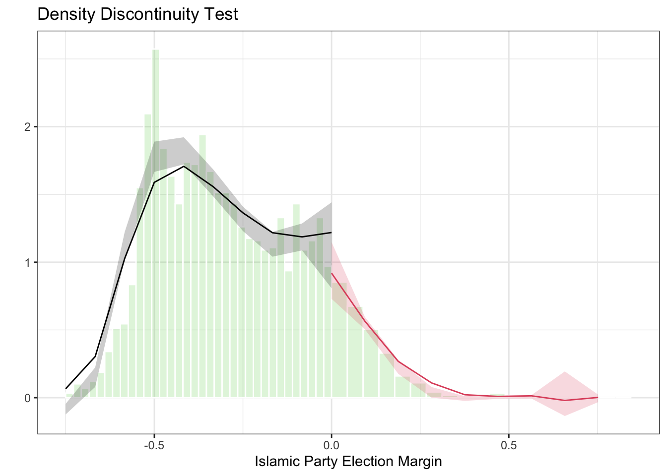

The robust p-value for the density discontinuity test is 0.36, meaning that we cannot reject the null hypothesis of no discontinuous jump in the density of the running variable at the cutoff. Visually, you can also see that there is no strong evidence of manipulation in the plot – the density estimates on either side of the cutoff appear to be continuous. This provides evidence supporting the validity of the RD design.

Note: the output also includes a table of binomial tests, which check whether the number of observations is balanced in symmetric windows around the cutoff. Some of these show significant p-values at wider windows, but this simply reflects the fact that the Islamic party lost in the majority of municipalities overall – it does not indicate manipulation at the cutoff. The relevant test is the robust density discontinuity test reported above.

Examine the sensitivity of the main RD result to the choice of bandwidth by calculating and plotting RD estimates and their associated 95% confidence intervals for a range of bandwidths from 0.05 to 0.6. To what extent do the results depend on the choice of bandwidth? Again, you could also plot this both for the conventional and robust estimates. Hint: You will need to use a loop to estimate the RD for each bandwidth since rdrobust doesn’t support passing a vector of bandwidths directly.

## Set-up the vector of bandwidths
bandwidths <- seq(from = 0.05, to = 0.6, by = 0.005)

## Setup storage vectors
est_c <- rep(NA, length(cut)) # conventional estimates
est_r <- rep(NA, length(cut)) # robust estimates
se_c <- rep(NA, length(cut)) # conventional standard errors
se_r <- rep(NA, length(cut)) # robust standard errors

## Loop over bandwidths
for (i in 1:length(bandwidths)) {
  rd_temp <- rdrobust(
    y = islamic$school_women, x = islamic$margin,
    c = 0, h = bandwidths[i]
  )
  
  est_c[i] <- rd_temp$coef[1] # conventional estimate
  se_c[i] <- rd_temp$se[1] # conventional standard error
  est_r[i] <- rd_temp$coef[3] # bias-corrected estimate
  se_r[i] <- rd_temp$se[3] # robust standard error
}

## Create data frame
results <- data.frame(
  bw = bandwidths,
  est_c = est_c,
  lo_c = est_c - 1.96 * se_c,
  hi_c = est_c + 1.96 * se_c,
  est_r = est_r,
  lo_r = est_r - 1.96 * se_r,
  hi_r = est_r + 1.96 * se_r,
  opt = abs(bandwidths - band) < 0.005
) # mark the optimal bandwidth

## plot
# conventional
p1 <- ggplot(results, aes(x = bw, y = est_c, color = opt)) +
  geom_linerange(aes(ymin = lo_c, ymax = hi_c), color = "gray") +
  geom_point() +
  geom_hline(yintercept = 0, linetype = "dotted") +
  scale_x_continuous("Bandwidth", breaks = seq(0.05, 0.6, .05)) +
  scale_color_manual(values = c("black", "red")) +
  ylab("Estimate") +
  ggtitle("Conventional estimates") +
  theme_clean() +
  lemon::coord_capped_cart(bottom = "both", left = "both") +
  theme(
    plot.background = element_rect(color = NA),
    panel.grid.major.y = element_blank(),
    legend.position = "none",
    axis.ticks.length = unit(2, "mm"))

# robust
p2 <- ggplot(results, aes(x = bw, y = est_r, color = opt)) +
  geom_linerange(aes(ymin = lo_r, ymax = hi_r), color = "gray") +
  geom_point() +
  geom_hline(yintercept = 0, linetype = "dotted") +
  scale_x_continuous("Bandwidth", breaks = seq(0.05, 0.6, .05)) +
  scale_color_manual(values = c("black", "red")) +
  ylab("Estimate") +
  ggtitle("Robust estimates") +
  theme_clean() +
  lemon::coord_capped_cart(bottom = "both", left = "both") +
  theme(
    plot.background = element_rect(color = NA),
    panel.grid.major.y = element_blank(),
    legend.position = "none",
    axis.ticks.length = unit(2, "mm"))

p1 / p2 + plot_annotation(title = "Placebo Tests: LATE Estimates at Different Bandwidths")

The plot shows a fairly typical pattern in RD analysis. At very low bandwidths, very little data is used in estimation, making the variance very high. Unsurprisingly therefore, the confidence interval is very wide at low bandwidths (recall that the MSE-optimal bandwidth is chosen with the twin goals of reducing both bias and variance). As the bandwidth (and therefore the effective sample size) increases, the confidence interval decreases.

The size of the RD estimate does not change much as the bandwidth increases, which is reassuring: we would not want our result to be extremely sensitive to the bandwidth choice. Its statistical significance does change somewhat as the bandwidth changes. For the conventional estimates, it is significant at the 95% level for bandwidths between approximately 0.15 and 0.5, becoming statistically indistinguishable from 0 at higher bandwidths. Note that the robust confidence intervals used here are wider than conventional ones, because they account for the additional uncertainty from bias correction. Nevertheless, the result holds across a reasonable range of bandwidths around the optimal one. It would not be very defensible to do RD estimation with a bandwidth much higher than 0.4 or so, where we are using data that is very far from the cutoff. Overall, if you saw this plot in a published paper you should feel reassured that the author’s results are not driven primarily by the choice of bandwidth.

9.2 Quiz

Why is a valid regression discontinuity design (RDD) able to overcome the typical problem of selection bias in observational designs?

Because it effectively eliminates bias from all confounders (observable and unobservable) for all units in the sample, allowing to estimate an unbiased ATE
Because it effectively removes all heterogeneity between treatment and control groups fixed over time and all time heterogeneity fixed across units, allowing to recover an unbiased ATT
Because it compares observed outcomes for units just below and just above a cutoff on a running variable. In a valid design, treatment assignment just above/below the cutoff is as good as random
Because it uses a weighted average of most similar untreated units as a counterfactual for the treated unit, allowing to construct a credible synthetic counterfactual

What assumptions does a sharp RDD require?

That the running variable is inducing at least some variation in the treatment condition (1\(^{st}\) stage assumption)
That potential outcomes evolve smoothly around the cutoff. Hence: no covariate is discontinuous around the cutoff and units cannot self-sort on either side
The strength of a sharp RDD is precisely that it requires no assumption at all, hence its high internal validity
That outcomes of units just below and just above the threshold would have followed the same time-trend, hadn’t it been for the treatment

What causal quantity is a sharp RDD estimating?

A local average treatment effect (LATE), which is specific to units with value of the running variable close to the cutoff, within a certain bandwidth
A local average treatment effect (LATE), which averages effects for units that are geographically proximate to each other, within a certain spatial bandwidth
A local average treatment effect (LATE), that relates only to units who comply with treatment assignment
A local average treatment effect (LATE), an extrapolation specific to units that are located precisely on the cutoff

How does enlarging the bandwidth affect an RDD?

Enlarging the bandwidth decreases the number of observations, increases external validity, and increases statistical power
Enlarging the bandwidth increases the number of observations, decreases internal validity, and increases statistical power
It is not possible to enlarge the bandwidth once an optimal value is selected with the optimal MSE algorithm
Enlarging the bandwidth increases the number of observations, decreases internal validity, and decreases statistical power

What is the procedure implemented by a fuzzy RDD?

Select covariates that are strongest in explaining the outcome variable. Give more weight to control units that are most similar to the treated unit with respect to them
Select, for each treated unit, the most similar untreated unit with respect to the included covariates. Keep only observations that satisfy this criterion and compute a difference in mean outcome
Restrict data within a bandwidth around the threshold. Code a treatment variable using the running variable. Fit a certain model (linear, multiplicative, polynomial, local linear). Take the coefficient of the treatment assignment as the estimated LATE
Restrict data within a bandwidth around the threshold. Code an instrument using the running variable. Proceed with a 2SLS procedure including the running variable in both stages. Take the coefficient of the fitted treatment assignment in the 2nd stage as the estimated LATE

Which of the following is NOT true about fuzzy RDD?

Units are assigned to treatment around the threshold, but not all units comply
The probability of treatment around the threshold is O on one side and 1 on the other
It requires only one identification assumption, the same as a sharp RDD
It combines regression discontinuity and instrumental variable estimation to overcome non-compliance with the treatment assignment at the threshold