R Refresher

If you are struggling to remember how R works since the last time you used it (which is reasonable: coding is like foreign language acquisition, if you don’t use it you lose it), then you might want to work through the exercises here. They are intended to remind you of some of the basics of coding in R, and using RStudio effectively.

We will cover the following topics:

Using R from the console
Using R from script files
Objects and assignment
Vectors
Functions
Help files
Data frames
Subsetting
Linear regression

RStudio

Let’s get acquainted with R and Rstudio. When you start RStudio for the first time, you’ll see three panels:

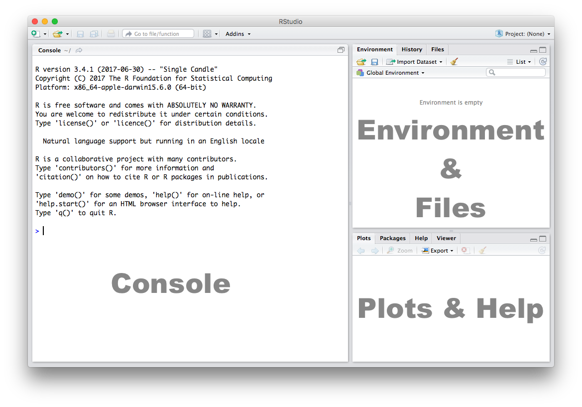
We will discuss what each of these does below.

Console

On the left is the console, which is the simplest way to interact with R. You can type some code at the console (click on the part where the cursor is > |) and when you press ENTER, R will run that code. Depending on what you type, you may see some output in the console or if you make a mistake, you may get a warning or an error message.

Let’s familiarize ourselves with the console by using R as a simple calculator:

2 + 4

## [1] 6

Now that we know how to use the + sign for addition, let’s try some other mathematical operations such as subtraction (-), multiplication (*), and division (/).

10 - 4

## [1] 6

5 * 3

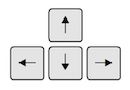
## [1] 15

7 / 2

## [1] 3.5

You can use the cursor or arrow keys on your keyboard to edit your code at the console:
- Use the UP and DOWN keys to re-run something without typing it again
- Use the LEFT and RIGHT keys to edit

Scripts

The Console is great for simple tasks but if you’re working on a project you would mostly likely want to save your work in some sort of a document or a file. Scripts in R are just plain text files that contain R code. You can edit a script just like you would edit a file in any word processing or note-taking application.

We recommend that you ALWAYS work from a script file in these classes.

Create a new script using the menu or the toolbar button as shown below.

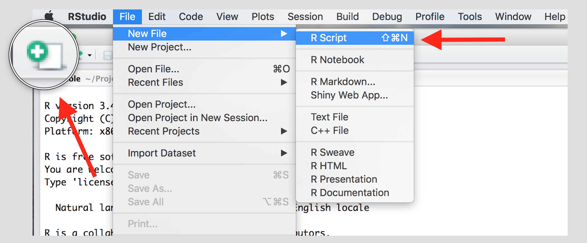
Once you’ve created a script, it is generally a good idea to give it a meaningful name and save it immediately.

Familiarize yourself with the script window in RStudio, and especially the two buttons labeled Run and Source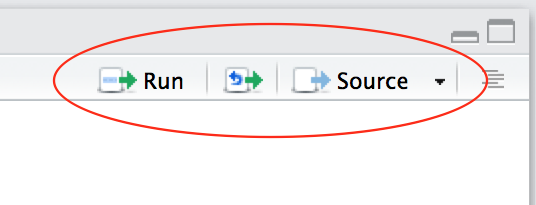

There are a few different ways to run your code from a script.

One line at a time	Place the cursor on the line you want to run and hit CTRL-ENTER or use the Run button
Multiple lines	Select the lines you want to run and hit CTRL-ENTER or use the Run button
Entire script	Use the Source button

Objects and assignment

The basic structures that R works with are called “objects”. Creating an object is simply a way of storing information in R, and we can give any object any name we like. Once we have created an object, we can use it in many other tasks later on.

Let’s begin by creating an object which stores the result of a simple addition. We use the assignment operator <- for creating or updating objects. If we wanted to save the result of adding 10 + 4, we would do the following:

my_result <- 10 + 4

The line above creates a new object called my_result in our environment and saves the result of the 10 + 4 in it. To see what’s in my_result, just type it at the console:

my_result

## [1] 14

Note that all object names are case-sensitive, so if you try entering My_Result at the console, you get:

## Error in eval(expr, envir, enclos): object 'My_Result' not found

The most useful thing about objects is that once they have been created, you can use them to perform subsequent calculations. For instance:

my_result*2

## [1] 28

You can even perform a calculation on an object and assign the result to a new object:

my_new_result <- my_result*2
my_new_result

## [1] 28

The possibilities are endless.

Now that we have created two objects, take a look at the Environment pane in RStudio and you’ll see both my_result and my_new_result there.

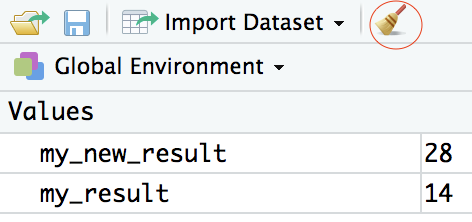
To delete all objects from the environment, you can use the broom button as shown in the picture above.

We called our object my_result but we can call it anything as long as we follow a few simple rules. Object names can contain upper or lower case letters (A-Z, a-z), numbers (0-9), underscores (_) or a dot (.) but all object names must start with a letter. Choose names that are descriptive and easy to type.

Good Object Names	Bad Object Names
result	a
my_result	x1
my.result	this.name.is.just.too.long
my_new_result	thing

Vectors

Both my_result and my_new_result are objects that contain single numbers. Frequently, we will want to work with long lists of numbers which are related to each other in some regard. The key building blocks we need for doing this are vectors. A vector is simply a set of information (normally numbers, but often also character strings or logical elements) contained together in a specific order.

One way to create a vector within R is to use the c() function, which “concatenates” many values together. For instance, we could concatenate the following numbers:

my_first_vector <- c(0, 1, 1, 2, 3, 5, 8, 13, 21, 34)
my_first_vector

##  [1]  0  1  1  2  3  5  8 13 21 34

The order in which the numbers in the vector are stored is important, and we can access individual elements of a vector by using square brackets, which look like this: [ ]. For instance, if we wish to access the 3rd element of the vector we just created, we can do the following

my_first_vector[3]

## [1] 1

This is a basic example of subsetting a vector so that we can access the part of it we would like to use. We can also use one vector to subset another, so that, for example, my_first_vector[c(1,3,5)] will return to us the first, third and fifth elements of our vector:

my_first_vector[c(1,3,5)]

## [1] 0 1 3

Functions

Functions are a set of instructions that carry out a specific task. Functions often require some input and generate some output. For example, instead of using the + operator for addition, we can use the sum function to add two or more numbers. Let’s try adding up all the elements in the vector that we created above.

sum(my_first_vector)

## [1] 88

Here we are providing our vector as the input to the sum() function and 88 is the output. You can check this manually if you like, or you can just trust that R is able to calculate the sum of those numbers.

A function always requires the use of parenthesis or round brackets (). Inputs to the function are called arguments and go inside the brackets. The output of a function is displayed on the screen but we can also have the option of saving the result of the output. For instance:

vec_sum <- sum(my_first_vector)
vec_sum

## [1] 88

Here, vec_sum is also an object! So we have performed a calculation (sum()) on some data (my_first_vector), and stored the result (vec_sum).

Try applying some other functions to the vector we have created. For instance, you could try mean(), median(), max(), and min(). Are the results what you expect them to be? Note that function names in R are case sensitive! That means that while mean(my_first_vector) will calculate the mean of your vector, Mean(my_first_vector) will produce an error.

Reveal answer

mean(my_first_vector)
median(my_first_vector)
max(my_first_vector)
min(my_first_vector)

## [1] 8.8
## [1] 4
## [1] 34
## [1] 0

Help

In the bottom-right of the console, you will see the panel which has tabs names Plots, Packages, Help, and Viewer. Most of these are not needed now, but let’s get to know the Help panel a little.

Any function that you use in R will have an associated help file. For example, if we wanted to know how to use the sum() function, we could type help(sum) and look at the online documentation.

help(sum)

The question mark ? can also be used as a shortcut to access online help.

?sum

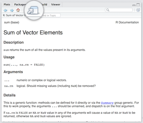
Use the toolbar button shown in the picture above to expand and display the help in a new window.

Help pages for functions in R follow a consistent layout and generally include these sections:

Description	A brief description of the function
Usage	The complete syntax or grammar including all arguments (inputs)
Arguments	Explanation of each argument
Details	Any relevant details about the function and its arguments
Value	The output value of the function
Examples	Example of how to use the function

data.frames

A data.frame is an object that holds data in a tabular format similar to how a spreadsheet works, where each column represents a variables and each row represents a unit.

Although you can create a data.frame manually, in most cases you will load a dataset from a file which will be represented in R as a data.frame. For now however, we will simply use a dataset that comes pre-installed with R.

Let’s take a look at a macroeconomic dataset called longley. To do so, run the following code in your R script:

data(longley)

The longley dataset is provided as a data frame of 7 variables and 16 observations.

help(longley)

The help screen describes each of the 7 variables. Now let’s see what’s in the longley dataset.

longley

##      GNP.deflator     GNP Unemployed Armed.Forces Population Year Employed
## 1947         83.0 234.289      235.6        159.0    107.608 1947   60.323
## 1948         88.5 259.426      232.5        145.6    108.632 1948   61.122
## 1949         88.2 258.054      368.2        161.6    109.773 1949   60.171
## 1950         89.5 284.599      335.1        165.0    110.929 1950   61.187
## 1951         96.2 328.975      209.9        309.9    112.075 1951   63.221
## 1952         98.1 346.999      193.2        359.4    113.270 1952   63.639
## 1953         99.0 365.385      187.0        354.7    115.094 1953   64.989
## 1954        100.0 363.112      357.8        335.0    116.219 1954   63.761
## 1955        101.2 397.469      290.4        304.8    117.388 1955   66.019
## 1956        104.6 419.180      282.2        285.7    118.734 1956   67.857
## 1957        108.4 442.769      293.6        279.8    120.445 1957   68.169
## 1958        110.8 444.546      468.1        263.7    121.950 1958   66.513
## 1959        112.6 482.704      381.3        255.2    123.366 1959   68.655
## 1960        114.2 502.601      393.1        251.4    125.368 1960   69.564
## 1961        115.7 518.173      480.6        257.2    127.852 1961   69.331
## 1962        116.9 554.894      400.7        282.7    130.081 1962   70.551

We can also look at the longley dataset graphically using the View function which displays the data frame like a spreadsheet.

View(longley)

Subsetting

For any data.frame we are analysing, we will often want to subset the data. That is, we will often wish to select only certain rows or certain columns from the data.

The `$` sign

The simplest way to access an individual column of a data.frame is to use the dollar sign $. For example, let’s see how to access the Year column:

longley$Year

##  [1] 1947 1948 1949 1950 1951 1952 1953 1954 1955 1956 1957 1958 1959 1960 1961
## [16] 1962

What is this? It is a vector! That is, it is a set of information joined together in an order. We can therefore access specific elements of our vector here just as we did with the example above. For example:

longley$Year[7]

## [1] 1953

The seventh element of the longley$Year vector is 1953.

Try using the dollar sign to access the GNP variable. What are the first, second, and tenth elements?

Reveal answer

longley$GNP

##  [1] 234.289 259.426 258.054 284.599 328.975 346.999 365.385 363.112 397.469
## [10] 419.180 442.769 444.546 482.704 502.601 518.173 554.894

longley$GNP[c(1,2,10)]

## [1] 234.289 259.426 419.180

square brackets `[,]`

We saw earlier that we can subset a vector by using square brackets: [ ]. When dealing with data.frames, we often want to access certain observations (rows) or certain columns (variables) or a combination of the two without looking at the entire dataset all at once. We can also use square brackets ([,]) to subset data frames.

In square brackets we put a row and a column coordinate separated by a comma. The row coordinate goes first and the column coordinate second. So longley[10, 3] returns the 10th row and third column of the data frame. If we leave the column coordinate empty this means we would like all columns. So, longley[10,] returns the 10th row of the dataset. If we leave the row coordinate empty, R returns the entire column. longley[,3] returns the third column of the dataset.

longley[10, 3] # element in 10th row, 3rd column

## [1] 282.2

longley[10, ] # entire 10th row

##      GNP.deflator    GNP Unemployed Armed.Forces Population Year Employed
## 1956        104.6 419.18      282.2        285.7    118.734 1956   67.857

longley[, 3] # entire 3rd column

##  [1] 235.6 232.5 368.2 335.1 209.9 193.2 187.0 357.8 290.4 282.2 293.6 468.1
## [13] 381.3 393.1 480.6 400.7

We can look at the first five rows of a dataset to get a better understanding of it with the colon in brackets like so: longley[1:5,]. We could display the second and fifth columns of the dataset by using the c() function in brackets like so: longley[, c(2,5)].

Display all columns of the longley dataset and show rows 10 to 15. Next display all columns of the dataset but only for rows 4 and 7.

Reveal answer

longley[10:15, ] # elements in 10th to 15th row, all columns

##      GNP.deflator     GNP Unemployed Armed.Forces Population Year Employed
## 1956        104.6 419.180      282.2        285.7    118.734 1956   67.857
## 1957        108.4 442.769      293.6        279.8    120.445 1957   68.169
## 1958        110.8 444.546      468.1        263.7    121.950 1958   66.513
## 1959        112.6 482.704      381.3        255.2    123.366 1959   68.655
## 1960        114.2 502.601      393.1        251.4    125.368 1960   69.564
## 1961        115.7 518.173      480.6        257.2    127.852 1961   69.331

longley[c(4, 7), ] # elements in 4th and 7th row, all columns

##      GNP.deflator     GNP Unemployed Armed.Forces Population Year Employed
## 1950         89.5 284.599      335.1        165.0    110.929 1950   61.187
## 1953         99.0 365.385      187.0        354.7    115.094 1953   64.989

Logical Operators

We can also subset by using logical values and logical operators. R has two special representations for logical values: TRUE and FALSE. R also has many logical operators, such as greater than (>), less than (<), or equal to (==).

When we apply a logical operator to an object, the value returned should be a logical value. For instance:

2 > 1

## [1] TRUE

2 < 1

## [1] FALSE

Here, when we ask R whether 2 is greater than 1, R returns the logical value TRUE. When we ask if 2 is less than 1, R returns the logical value FALSE.

For the purposes of subsetting, logical operations are useful because they can be used to specify which elements of a vector or data.frame we would like returned. For instace, say we would like to use only longley data from 1955 onwards. To subset the data to these observations, we can do the following:

longley[longley$Year > 1954,]

##      GNP.deflator     GNP Unemployed Armed.Forces Population Year Employed
## 1955        101.2 397.469      290.4        304.8    117.388 1955   66.019
## 1956        104.6 419.180      282.2        285.7    118.734 1956   67.857
## 1957        108.4 442.769      293.6        279.8    120.445 1957   68.169
## 1958        110.8 444.546      468.1        263.7    121.950 1958   66.513
## 1959        112.6 482.704      381.3        255.2    123.366 1959   68.655
## 1960        114.2 502.601      393.1        251.4    125.368 1960   69.564
## 1961        115.7 518.173      480.6        257.2    127.852 1961   69.331
## 1962        116.9 554.894      400.7        282.7    130.081 1962   70.551

What is happening here? It is worth going through this code slowly:

We are using the $ sign to extract the variable Year from the data.frame longley
We are asking R to tell us which observations of that variable are greater than 1954
We are subsetting the data.frame longley using the [,] to only the observations that match that condition

We can see a little more detail if we just evaluate the code that is within the square parenthesis:

longley$Year > 1954

##  [1] FALSE FALSE FALSE FALSE FALSE FALSE FALSE FALSE  TRUE  TRUE  TRUE  TRUE
## [13]  TRUE  TRUE  TRUE  TRUE

As you can see, R is returning a value of TRUE for the observations where Year is greater than 1954, and it is returning FALSE otherwise. It is this “logical” vector that is being used within the square brackets to subset the data.frame.

Now you can try! Use a logical operator to subset the longley data to only those observations where the population is smaller than 115.

Reveal answer

longley[longley$Population < 115, ]

##      GNP.deflator     GNP Unemployed Armed.Forces Population Year Employed
## 1947         83.0 234.289      235.6        159.0    107.608 1947   60.323
## 1948         88.5 259.426      232.5        145.6    108.632 1948   61.122
## 1949         88.2 258.054      368.2        161.6    109.773 1949   60.171
## 1950         89.5 284.599      335.1        165.0    110.929 1950   61.187
## 1951         96.2 328.975      209.9        309.9    112.075 1951   63.221
## 1952         98.1 346.999      193.2        359.4    113.270 1952   63.639

Putting it all together

Now that we have learned about functions, subsetting, and object assignment, we can combine these three things. Let’s try comparing the mean GNP levels in the US before and after 1955. Try using the tools you have learned above to do this before looking at the answer below.

Reveal answer

mean_gnp_pre_55 <- mean(longley[longley$Year < 1955,]$GNP)
mean_gnp_post_55 <- mean(longley[longley$Year >= 1955,]$GNP)

mean_gnp_pre_55
mean_gnp_post_55

## [1] 305.1049
## [1] 470.292

What is happening in this code? For the first line of the results above, we can describe each step as follows:

longley$Year < 1955 selects the rows of longley for which the variable Year is smaller than 1955
$GNP selects the GNP variable
mean() calculates the mean of that variable
mean_gnp_pre_55 <- assigns the result of that calculation to the object mean_gnp_pre_55

We are then simply repeating the same steps for a different subset of data on the second line, where longley$Year >= 1955 selects the rows where Year is greater than or equal to 1955.

Linear regression

Linear regression is implemented in R using the lm() function. The lm() function needs to know a) the relationship we’re trying to model and b) the dataset that contains our observations. The two arguments we need to provide to the lm() function are described below.

`lm` function arguments
Argument	Description
`formula`	The `formula` describes the relationship between the dependent and independent variables, for example `dependent.variable ~ independent.variable`
`data`	This is simply the name of the dataset that contains the variable of interest.

For more information on how the lm() function works, type help(lm) in R.

Continuing from the example above, run a linear regression where GNP is your outcome variable and your independent variable is binary, equal to 1 when Year is greater than or equal to 1955 and 0 otherwise (you will need to code this variable yourself). Again, try to do this for yourself before looking at the solution below.

Reveal answer

# Code the binary independent variable
longley$post_1955 <- longley$Year >= 1955

# Run the regression
gnp_ols <- lm(GNP ~ post_1955, longley)

# Summarise the results
summary(gnp_ols)

## 
## Call:
## lm(formula = GNP ~ post_1955, data = longley)
## 
## Residuals:
##     Min      1Q  Median      3Q     Max 
## -72.823 -46.022  -4.047  43.391  84.602 
## 
## Coefficients:
##               Estimate Std. Error t value Pr(>|t|)    
## (Intercept)     305.10      18.67  16.341 1.63e-10 ***
## post_1955TRUE   165.19      26.40   6.256 2.11e-05 ***
## ---
## Signif. codes:  0 '***' 0.001 '**' 0.01 '*' 0.05 '.' 0.1 ' ' 1
## 
## Residual standard error: 52.81 on 14 degrees of freedom
## Multiple R-squared:  0.7365, Adjusted R-squared:  0.7177 
## F-statistic: 39.14 on 1 and 14 DF,  p-value: 2.105e-05

As you can see, the coefficient on the regression - 165.19 - is the same as the difference in means that you calculated “manually” above.

mean_gnp_post_55 - mean_gnp_pre_55

## [1] 165.1871

T-tests

Let’s calculate the difference in means one final time, this using the the t-test function t.test(). The syntax of the function is:

t.test(formula, mu, alt, conf)

This function takes the following arguments

`t.test` function arguments
Arguments	Description
`formula`	The formula describes the relationship between the dependent and independent variables, for example: • `dependent.variable ~ independent.variable`. We will do this in the t-test for the difference in means.
`mu`	Here, we set the null hypothesis. The null hypothesis is that the true difference in means in the population mean is 0. Thus, we set `mu = 0`.
`alt`	There are two alternatives to the null hypothesis that the difference in means is zero. The difference could either be smaller or it could be larger than zero. To test against both alternatives, we set `alt = "two.sided"`.
`conf`	Here, we set the level of confidence that we want in rejecting the null hypothesis. Common confidence intervals are: 95%, 99%, and 99.9%.

Use the t-test function to compare the mean level of GNP in pre- and post-1955 years. Again, try to do this for yourself before looking at the solution below.

Reveal answer

t.test(longley$GNP ~ longley$post_1955, mu = 10000, alt = "two.sided")

## 
##  Welch Two Sample t-test
## 
## data:  longley$GNP by longley$post_1955
## t = -384.98, df = 13.992, p-value < 2.2e-16
## alternative hypothesis: true difference in means between group FALSE and group TRUE is not equal to 10000
## 95 percent confidence interval:
##  -221.8222 -108.5521
## sample estimates:
## mean in group FALSE  mean in group TRUE 
##            305.1049            470.2920

The results are, of course, identical to those we calculated above.

Further exercises

Create a folder with the name POLS0012 on your computer. Store all your work for this course in this folder for the rest of the term.
Create a new file called r_refresher.R in your POLS0012 folder and write all the solutions for this homework in it.
In the script that you have created, calculate the square root of 1369 using the sqrt() function.

Solution

sqrt(1369)

## [1] 37

Square the number 13 using the ^ operator.

Solution

13^2

## [1] 169

What is the result of summing all numbers from 1 to 100? Rather than typing all the numbers out, try using 1:100, which will give you the sequence of integers between 0 and 100.

Solution

sum(1:100)

## [1] 5050

Working with data

Let’s make use of another dataset that comes preloaded with R. Start by loading this data into your environment:

data(USArrests)

The USArrests data contains statistics on various violent crimes in each of the 50 US states in 1973.

Answer the following questions:

What are the variables contained in this data?

Solution

There are a number of ways of finding out this information. You could use the help() function, which would provide you with a full description of the data. Or you could use head() to see the first 6 rows of the data, or View() to open the data in a spreadsheet-style browser window. Let’s use head() for now:

head(USArrests)

##            Murder Assault UrbanPop Rape
## Alabama      13.2     236       58 21.2
## Alaska       10.0     263       48 44.5
## Arizona       8.1     294       80 31.0
## Arkansas      8.8     190       50 19.5
## California    9.0     276       91 40.6
## Colorado      7.9     204       78 38.7

The data contains four variables: the number of murders, assaults and rapes per 100,000 state residents, and the percentage of the urban population in each state. (Details on the scales of these variables can be found in the accompanying help file.)

Calculate the mean and median of each of the variables included in the data. Assign each of the results of these calculations to objects with sensible names.

Solution

mean_murders <- mean(USArrests$Murder)
median_murders <- median(USArrests$Murder)

mean_assault <- mean(USArrests$Assault)
median_assault <- median(USArrests$Assault)

mean_urban <- mean(USArrests$UrbanPop)
median_urban <- median(USArrests$UrbanPop)

mean_rape <- mean(USArrests$Rape)
median_rape <- median(USArrests$Rape)

Is there a difference in the assualt rate for urban and rural states? Define an urban state as one for which the urban population is greater than or equal to the median across all states. Define a rural state as one for which the urban population is less than the median. Use the coding techniques covered in class to answer this question. Once you have calculated the relevant numbers, write a sentence communicating your findings in substantive terms.

Solution

This question requires you to subset the data to those states with high and low urban populations, where high is states above the median urban population and low is states below the median urban population.

mean_assault_high_urban <- mean(USArrests[USArrests$UrbanPop >= median_urban,]$Assault)
mean_assault_low_urban <- mean(USArrests[USArrests$UrbanPop < median_urban,]$Assault)

This code is very similar to the code we covered at the end of the seminar. We use a logical operator (>=) to subset the data according to whether the UrbanPop variable is greater than or equal to median_urban. We then calculate the mean assault rate. We then do the same for states with an urban population below the median.

In substantive terms, these results suggest that, on average, states with high urban populations have a higher per capita assault rate than states with low urban populations. Specifically, the average assault rate for high urban states is 187 per 100,000, and it is only 150 per 100,000 for low urban states.

Final things

Save your script! You should now have all the answers to all the exercises in the same place.
“Source” your script, i.e. run the entire script all at once. Fix the script if you get any error messages.

R Refresher

RStudio

Console

Scripts

Objects and assignment

Vectors

Functions

Help

data.frames

Subsetting

The $ sign

square brackets [,]

Logical Operators

Putting it all together

Linear regression

T-tests

Further exercises

Working with data

Final things

The `$` sign

square brackets `[,]`