1 Introduction to Quantitative Analysis

1.1 Seminar

1.1.1 Getting Started

Install R and RStudio on your computer by downloading them from the following sources:

Download R from The Comprehensive R Archive Network (CRAN)
Download RStudio from RStudio.com

1.1.2 RStudio

Let’s get acquainted with R. When you start RStudio for the first time, you’ll see three panes:

1.1.3 Courseware Setup

We’ll get started by typing the following at the console to install the courseware:

source("https://uclspp.github.io/PUBLG100/R/setup_courseware.R")

When the setup app starts, press the Setup Courseware button to install the necessary files. If you run into any problems, you can click on the Help tab and send an error report.

If you’re unable to download the datasets using the setup app, you can manually download them from https://uclspp.github.io/datasets.

1.1.4 Console

The Console in RStudio is the simplest way to interact with R. You can type some code at the Console and when you press ENTER, R will run that code. Depending on what you type, you may see some output in the Console or if you make a mistake, you may get a warning or an error message.

Let’s familiarize ourselves with the console by using R as a simple calculator:

2 + 4

[1] 6

Now that we know how to use the + sign for addition, let’s try some other mathematical operations such as subtraction (-), multiplication (*), and division (/).

10 - 4

[1] 6

5 * 3

[1] 15

7 / 2

[1] 3.5

You can use the cursor or arrow keys on your keyboard to edit your code at the console:
- Use the UP and DOWN keys to re-run something without typing it again
- Use the LEFT and RIGHT keys to edit

Take a few minutes to play around at the console and try different things out. Don’t worry if you make a mistake, you can’t break anything easily!

1.1.5 Functions

Functions are a set of instructions that carry out a specific task. Functions often require some input and generate some output. For example, instead of using the + operator for addition, we can use the sum function to add two or more numbers.

sum(1, 4, 10)

[1] 15

In the example above, 1, 4, 10 are the inputs and 15 is the output. A function always requires the use of parenthesis or round brackets (). Inputs to the function are called arguments and go inside the brackets. The output of a function is displayed on the screen but we can also have the option of saving the result of the output. More on this later.

1.1.6 Getting Help

Another useful function in R is help which we can use to display online documentation. For example, if we wanted to know how to use the sum function, we could type help(sum) and look at the online documentation.

help(sum)

The question mark ? can also be used as a shortcut to access online help.

?sum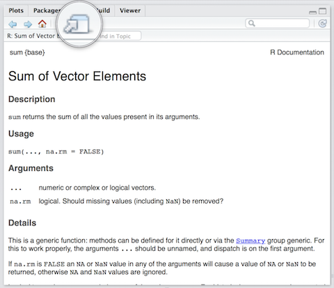

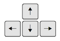
Use the toolbar button shown in the picture above to expand and display the help in a new window.

Help pages for functions in R follow a consistent layout generally include these sections:

Desscription	A brief description of the function
Usage	The complete syntax or grammar including all arguments (inputs)
Arguments	Explanation of each argument
Details	Any relevant details about the function and its arguments
Value	The output value of the function
Examples	Example of how to use the function

1.1.7 The Assignment Operator

Now we know how to provide inputs to a function using parenthesis or round brackets (), but what about the output of a function?

We use the assignment operator <- for creating or updating objects. If we wanted to save the result of adding sum(1, 4, 10), we would do the following:

myresult <- sum(1, 4, 10)

The line above creates a new object called myresult in our environment and saves the result of the sum(1, 4, 10) in it. To see what’s in myresult, just type it at the console:

myresult

[1] 15

Take a look at the Environment pane in RStudio and you’ll see myresult there.

To delete all objects from the environment, you can use the broom button as shown in the picture above.

We called our object myresult but we can call it anything as long as we follow a few simple rules. Object names can contain upper or lower case letters (A-Z, a-z), numbers (0-9), underscores (_) or a dot (.) but all object names must start with a letter. Choose names that are descriptive and easy to type.

Good Object Names	Bad Object Names
result	a
myresult	x1
my.result	this.name.is.just.too.long
my_result
data1

1.1.8 Sequences

We often need to create sequences when manipulating data. For instance, you might want to perform an operation on the first 10 rows of a dataset so we need a way to select the range we’re interested in.

There are two ways to create a sequence. Let’s try to create a sequence of numbers from 1 to 10 using the two methods:

Using the colon : operator. If you’re familiar with spreadsheets then you might’ve already used : to select cells, for example A1:A20. In R, you can use the : to create a sequence in a similar fashion:

1:10

 [1]  1  2  3  4  5  6  7  8  9 10

Using the seq function we get the exact same result:

seq(1, 10)

 [1]  1  2  3  4  5  6  7  8  9 10

The seq function has a number of options which control how the sequence is generated. For example to create a sequence from 0 to 100 in increments of 5, we can use the optional by argument. Notice how we wrote by = 5 as the third argument. It is a common practice to specify the name of argument when the argument is optional.

seq(0, 100, by = 5)

 [1]   0   5  10  15  20  25  30  35  40  45  50  55  60  65  70  75  80
[18]  85  90  95 100

Take a look at the help page for seq to see what other options are available.

help(seq)

Now it’s your turn:

Create a sequence of odd numbers between 0 and 100 and save it in an object called odd_numbers

odd_numbers <- seq(1, 100, 2)

Next, display odd_numbers on the console to verify that you did it correctly

odd_numbers

 [1]  1  3  5  7  9 11 13 15 17 19 21 23 25 27 29 31 33 35 37 39 41 43 45
[24] 47 49 51 53 55 57 59 61 63 65 67 69 71 73 75 77 79 81 83 85 87 89 91
[47] 93 95 97 99

What do the numbers in square brackets [ ] mean? Look at the number of values displayed in each line to find out the answer.
Use the length function to find out how many values are in the object odd_numbers.
- HINT: Try help(length) and look at the examples section at the end of the help screen.

length(odd_numbers)

[1] 50

1.1.9 Scripts

The Console is great for simple tasks but if you’re working on a project you would mostly likely want to save your work in some sort of a document or a file. Scripts in R are just plain text files that contain R code. You can edit a script just like you would edit a file in any word processing or note-taking application.

Create a new script using the menu or the toolbar button as shown below.

Once you’ve created a script, it is generally a good idea to give it a meaningful name and save it immediately. For our first session save your script as seminar1.R

Familiarize yourself with the script window in RStudio, and especially the two buttons labeled Run and Source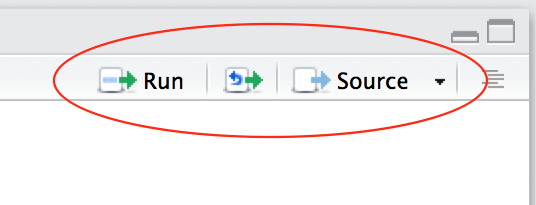

There are a few different ways to run your code from a script.

One line at a time	Place the cursor on the line you want to run and hit CTRL-ENTER or use the Run button
Multiple lines	Select the lines you want to run and hit CTRL-ENTER or use the Run button
Entire script	Use the Source button

1.1.10 data frames

A data frame is an object that holds data in a tabular format similar to how spreadsheets work. Variables are generally kept in columns and observations are in rows.

Although you can create a data frame manually, in most cases you will create a data frame by loading a dataset from a file. For now however, we will simply use a dataset that comes pre-installed with R.

Let’s take a look at a macroeconomic dataset called longley. The longley dataset is provided as a data frame of 7 variables and 16 observations.

help(longley)

The help screen describes each of the 7 variables. Now let’s see what’s in the longley dataset.

longley

     GNP.deflator     GNP Unemployed Armed.Forces Population Year Employed
1947         83.0 234.289      235.6        159.0    107.608 1947   60.323
1948         88.5 259.426      232.5        145.6    108.632 1948   61.122
1949         88.2 258.054      368.2        161.6    109.773 1949   60.171
1950         89.5 284.599      335.1        165.0    110.929 1950   61.187
1951         96.2 328.975      209.9        309.9    112.075 1951   63.221
1952         98.1 346.999      193.2        359.4    113.270 1952   63.639
1953         99.0 365.385      187.0        354.7    115.094 1953   64.989
1954        100.0 363.112      357.8        335.0    116.219 1954   63.761
1955        101.2 397.469      290.4        304.8    117.388 1955   66.019
1956        104.6 419.180      282.2        285.7    118.734 1956   67.857
1957        108.4 442.769      293.6        279.8    120.445 1957   68.169
1958        110.8 444.546      468.1        263.7    121.950 1958   66.513
1959        112.6 482.704      381.3        255.2    123.366 1959   68.655
1960        114.2 502.601      393.1        251.4    125.368 1960   69.564
1961        115.7 518.173      480.6        257.2    127.852 1961   69.331
1962        116.9 554.894      400.7        282.7    130.081 1962   70.551

We can also look at the longley dataset graphically using the View function which displays the data frame like a spreadsheet.

View(longley)

In order to access individual columns of a data frame we use the dollar sign $. For example, let’s see how to access the Year column

longley$Year

 [1] 1947 1948 1949 1950 1951 1952 1953 1954 1955 1956 1957 1958 1959 1960
[15] 1961 1962

Often we want to access certain observations (rows) or certain columns (variables) or a combination of the two without looking at the entire dataset all at once. We can use square brackets to subset data frames. In square brackets we put a row and a column coordinate separated by a comma. The row coordinate goes first and the column coordinate second. So longley[10, 3] returns the 10th row and third column of the data frame. If we leave the column coordinate empty this means we would like all columns. So, longley[10,] returns the 10th row of the dataset. If we leave the row coordinate empty, R returns the entire column. longley[,3] returns the third column of the dataset.

longley[10, 3] # element in 10th row, 3rd column

[1] 282.2

longley[10, ] # entire 10th row

     GNP.deflator    GNP Unemployed Armed.Forces Population Year Employed
1956        104.6 419.18      282.2        285.7    118.734 1956   67.857

longley[, 3] # entire 3rd column

 [1] 235.6 232.5 368.2 335.1 209.9 193.2 187.0 357.8 290.4 282.2 293.6
[12] 468.1 381.3 393.1 480.6 400.7

We can look at the first five rows of a dataset to get a better understanding of it with the colon in brackets like so: longley[1:5,]. We could display the second and fifth columns of the dataset by using the c() function in brackets like so: longley[, c(2,5)].

It’s your turn. Display all columns of the longley dataset and show rows 10 to 15. Next display all columns of the dataset and rows 4 and 7.

longley[10:15, ] # elements in 10th to 15th row, all columns

     GNP.deflator     GNP Unemployed Armed.Forces Population Year Employed
1956        104.6 419.180      282.2        285.7    118.734 1956   67.857
1957        108.4 442.769      293.6        279.8    120.445 1957   68.169
1958        110.8 444.546      468.1        263.7    121.950 1958   66.513
1959        112.6 482.704      381.3        255.2    123.366 1959   68.655
1960        114.2 502.601      393.1        251.4    125.368 1960   69.564
1961        115.7 518.173      480.6        257.2    127.852 1961   69.331

longley[c(4, 7), ] # elements in 4th and 7th row, all column

     GNP.deflator     GNP Unemployed Armed.Forces Population Year Employed
1950         89.5 284.599      335.1        165.0    110.929 1950   61.187
1953         99.0 365.385      187.0        354.7    115.094 1953   64.989

1.1.11 Plots

Now let’s create some plots from the longley dataset. First let’s create a scatterplot with the Year variable on the x-axis and Employed on the y-axis.

plot(longley$Year, longley$Employed)

To create a line plot instead, we use the same function with one additional argument type = "l".

plot(longley$Year, longley$Employed, type = "l")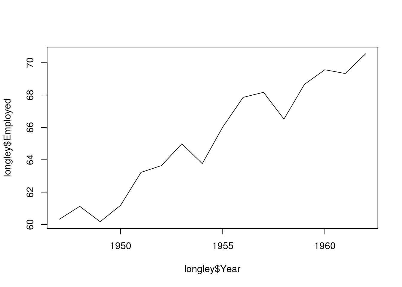

Now it’s your turn.

Use online help for the plot function and find out how to create a plot that includes both points and lines.

plot(longley$Year, longley$Employed, type = "b")

1.1.12 Exercises

Create a script and call it assignment01. Save your script.
Download this cheat-sheet and go over it. You won’t understand most of it right a away. But it will become a useful resource. Look at it often.
Calculate the square root of 1369 using the sqrt() function.
Square the number 13 using the ^ operator.
What is the result of summing all numbers from 1 to 100?
Use the names() function to display the variable names of the longley dataset.
Use square brackets to access the 4th column of the dataset.
Use the dollar sign to access the 4th column of the dataset.
Access the two cells from row 4 and column 1 and row 6 and column 3.
Using the longley data produce a line plot with GNP on the y-axis and population on the x-axis.
Use the help function to find out how to label the y-axis “wealth” and the x-axis “population”.
Save your script, which should now include the answers to all the exercises.
Source your script, i.e. run the entire script without error message. Clean your script if you get error messages.