2.2 Solutions
2.2.1 Exercise 2
Clear the workspace and set the working directory to your PUBLG100 folder.
# clear workspace
rm(list = ls())
# set working directory
setwd("~/PUBLG100")
2.2.2 Exercise 3
Load the non-western foreigners dataset from your local drive into R.
load("non_western_foreingners.RData")2.2.3 Exercise 4
What is the level of measurement for each variable in the non-western foreigners dataset?
IMMBRITis interval scaled (continuous).over.estimateis categorical with 2 categories, also called a binary variable, a dummy variable, or an indicator variable.Rsexis categorical as well with 2 categories.RAgeis interval scaled.Househldis interval scaled.paperis categorical with 2 categories.WWWhourspWis interval scaled.religiousis categorical with 2 categories.employMonthsis interval scaled.urbanis an ordinal variable.health.goodis an ordinally scaled variable.HHIncWe do not have enough information to determine whether HHInc is interval scaled or ordinal. If the income bands are equally large,HHIncwould be interval scaled. We will treat the variable as interval scaled.
2.2.4 Exercise 5
Calculate the correct measure of central tendency for RAge, Househld, religious.
The correct measures of central tendency for the three levels of measurement are:
| level_of_measurement | central_tendency |
|---|---|
| categorical | Mode |
| ordinal | Median |
| interval | Mean |
mean(fdata$RAge)[1] 49.74547mean(fdata$Househld)[1] 2.391802mean(fdata$religious)[1] 0.4928503The mean of age is 49.7, the mean of Househeld is 2.4. The mode of religious is 0.
Note: Because religious is binary, taking the mean tells us what the mode is because we know the proportion of 1’s. 49% are religious, therefore, more people are not religious.
2.2.5 Exercise 6
Calculate the correct measure of dispersion for RAge, Househld, religious.
sd(fdata$RAge)[1] 17.57245sd(fdata$Househld)[1] 1.339352mean(fdata$religious)[1] 0.4928503The standard deviation of age is 17.6, the standard deviation of the number of people in the respondents household is 1.3. 49% of the respondents are religious and 51% are not.
2.2.6 Exercise 7
How many respondents identify with the Greens?
fdata$party_self <- factor(fdata$party_self, labels = c("Tories", "Labour", "SNP", "Greens", "Ukip", "BNP", "other"))

# first solution, just look at the frequency table
table(fdata$party_self)
Tories Labour    SNP Greens   Ukip    BNP  other
   284    280     16     23     31     32    383
# another solution using the which() function
length(which(fdata$party_self=="Greens"))[1] 2323 respondents identify with the Green party.
2.2.7 Exercise 8
Calculate the variance and standard deviation of IMMBRIT for each party affiliation.
# conservatives
var(fdata$IMMBRIT[fdata$party_self=="Tories"])
[1] 431.8308sd(fdata$IMMBRIT[fdata$party_self=="Tories"])[1] 20.78054# labour
var(fdata$IMMBRIT[fdata$party_self=="Labour"])[1] 444.8932sd(fdata$IMMBRIT[fdata$party_self=="Labour"])[1] 21.09249# snp
var(fdata$IMMBRIT[fdata$party_self=="SNP"])[1] 145sd(fdata$IMMBRIT[fdata$party_self=="SNP"])[1] 12.04159# greens
var(fdata$IMMBRIT[fdata$party_self=="Greens"])[1] 591.8103sd(fdata$IMMBRIT[fdata$party_self=="Greens"])[1] 24.32715# ukip
var(fdata$IMMBRIT[fdata$party_self=="Ukip"])[1] 288.2796sd(fdata$IMMBRIT[fdata$party_self=="Ukip"])[1] 16.9788# bnp
var(fdata$IMMBRIT[fdata$party_self=="BNP"])[1] 657.1895sd(fdata$IMMBRIT[fdata$party_self=="BNP"])[1] 25.63571# other
var(fdata$IMMBRIT[fdata$party_self=="other"])[1] 434.8236sd(fdata$IMMBRIT[fdata$party_self=="other"])[1] 20.852422.2.8 Exercise 9
Find the party affiliation of the oldest and youngest respondents.
# max and min ages
range(fdata$RAge)
[1] 17 99# row index numbers of oldest and youngest respondents
oldest <- which(fdata$RAge == max(fdata$RAge))
youngest <- which(fdata$RAge == min(fdata$RAge))
# party affiliation of those respondents
fdata$party_self[oldest][1] other Labour
Levels: Tories Labour SNP Greens Ukip BNP otherfdata$party_self[youngest][1] other
Levels: Tories Labour SNP Greens Ukip BNP otherTwo respondents were 99 years old. One identifies with a party other than the six parties we listed, and the other respondent indentifies with Labour.
The youngest respondent is 17 and identifies with a party other than the six we listed.
2.2.9 Exercise 10
Find the 20th, 40th, 60th and 80th percentiles of RAge.
quantile(fdata$RAge, c(.2, .4, .6, .8))20% 40% 60% 80%
33 44 55 66 2.2.10 Exercise 11
Create a box plot for IMMBRIT grouped by the paper variable to show the difference between IMMBRIT for people who read daily morning newspapers three or more times per week and people who do not.
boxplot( IMMBRIT ~ paper, data = fdata)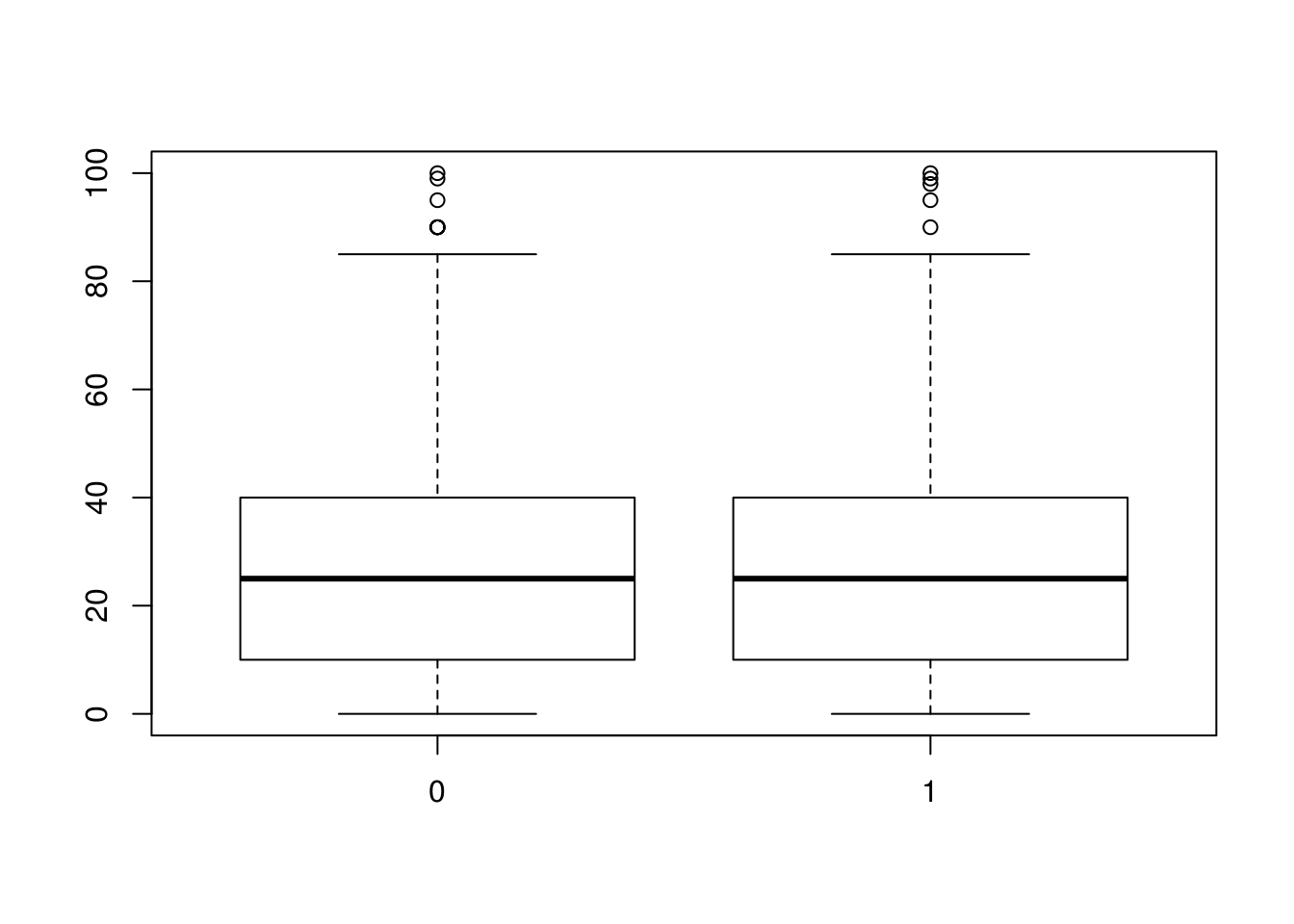
The two conditional distributions look identical. This plot shows no difference in the subjective number of immigrants for people who read daily morning newspapers and people who do not.
2.2.11 Exercise 12
What is the mean of IMMBRIT for men and for women?
# men
mean(fdata$IMMBRIT[fdata$RSex==1])
[1] 24.53766# women
mean(fdata$IMMBRIT[fdata$RSex==2])[1] 32.79159The mean for men is 24.5 and the mean for women is 32.9
2.2.12 Exercise 13
What is the numerical difference between those two means?
mean(fdata$IMMBRIT[fdata$RSex==2]) - mean(fdata$IMMBRIT[fdata$RSex==1])[1] 8.253937The difference in means between women and men is 8.3 or put differently: women overestimate the number of immigrants more than men. The difference seems to be quite large 8.3 per 100 (8.3 percentage points).