9.2 Solutions
9.2.0.1 Exercise 1
- Load the non-western foreigners dataset non_western_foreingners.RData from your PUBLG 100 folder.
rm(list = ls())
load("non_western_foreingners.RData")- Build a model that predicts
over.estimateto find determinants of over-estimating the level of migration. Justify your choice of predictors and interpret the model output.
We choose RAge, and party_self as predictors. Party identification is linked to the ideology of a respondent which likely predicts whether someone over estimates the level of migration. The more right leaning the party the respondent identifies with, the more likely she is to over estimate. Similarly, older respondents are expected to be more likely to over estimate because they could be more opposed to change and, therefore, have an incentive to over estimate.
m1 <- glm(over.estimate ~ RAge + as.factor(party_self), data = fdata, family = binomial(link="logit"))
library(texreg)
screenreg(m1)
=================================
                        Model 1
---------------------------------
(Intercept)                0.46
                          (0.25)
RAge                       0.01
                          (0.00)
as.factor(party_self)2     0.03
                          (0.18)
as.factor(party_self)3     1.93
                          (1.04)
as.factor(party_self)4    -0.33
                          (0.45)
as.factor(party_self)5     0.23
                          (0.43)
as.factor(party_self)6     1.23 *
                          (0.55)
as.factor(party_self)7     0.32
                          (0.18)
---------------------------------
AIC                     1236.01
BIC                     1275.65
Log Likelihood          -610.00
Deviance                1220.01
Num. obs.               1049
=================================
*** p < 0.001, ** p < 0.01, * p < 0.05- What is the naive guess of
over.estimate?
table(fdata$over.estimate)
  0   1
290 759
759 people over estimate, more than the 290 who do not. The naive guess is over.estimate = 1, i.e. people over estimate.
- What is the percentage of correctly predicted cases using the naive guess?
759 / (290 + 759)[1] 0.7235462If we predict that everyone over estimates, we get \(759\) cases out of \(759+290=1049\) right. That is \(759/1049=72\%\).
- What is the percent of correctly predicted cases of your model and how does it compare to the naive guess?
# predicted probs
fdata$pp <- predict(m1, type = "response")

# expected values
fdata$evs <- ifelse(fdata$pp > .5, yes = 1, no = 0)

# confusion matrix
table(actual = fdata$over.estimate, predictions = fdata$evs)
predictions
actual 1
0 290
1 759A quick look at the confusion table shows, our makes no contribution. It predicts over.estimate = 1 for everyone in the data. That is the same as the naive guess.
- Add predictors to your model and justify the choice.
We control for the degree of urbanization. Urban areas are more liberal and have less of an incentive to over estimate. Furthermore, we control for income. Richer respondents tend to be more educated and thus have a more accurate idea about levels of migration and migrants do not compete with them. Therefore, they have less of an incentive to over estimate. In addition, we control for gender, because men might be more conservative and tend to over estimate more.
m2 <- glm(over.estimate ~ RAge + as.factor(party_self) + RSex + HHInc + as.factor(urban),
data = fdata, family = binomial(link = "logit")) - Are the added predictors jointly significant?
We use the likelihood ratio test.
library(lmtest)
lrtest(m1, m2)
Likelihood ratio test
Model 1: over.estimate ~ RAge + as.factor(party_self)
Model 2: over.estimate ~ RAge + as.factor(party_self) + RSex + HHInc +
as.factor(urban)
#Df LogLik Df Chisq Pr(>Chisq)
1 8 -610.00
2 13 -572.95 5 74.105 1.43e-14 ***
---
Signif. codes: 0 '***' 0.001 '**' 0.01 '*' 0.05 '.' 0.1 ' ' 1The coefficients of the added variables are jointly significant. Our p value is less than \(0.05\).
- What is the new rate of correctly predicted cases? Is it better than the first model and how does it compare to the naive guess?
# predicted probs
fdata$pp2 <- predict(m2, type = "response")
# expected values
fdata$evs2 <- ifelse(fdata$pp2 > 0.5, 1, 0)
# crosstable predictions against real outcomes
table(actual = fdata$over.estimate, predictions = fdata$evs2)
predictions
actual 0 1
0 43 247
1 32 727Our new model improves upon model 1. In model 1, we made \(759\) correct predictions. In our new model, we are up to \(43+727=770\). The percentage of correct predictions is:
(43+727) / (43 + 247 + 32 + 727 )[1] 0.7340324\(73\%\). We improve by 1 percentage point, a marginal improvement.
- Vary the threshold for generating expected values and compute the percent correctly predicted cases again. How does it change?
Varying the threshold only makes sense if we care about the types of errors we make. Let’s say, in our world false positives are worse than false negatives. We could try to reduce the number of false positive mistakes we are making by increasing the threshold. The intution is that if before we classified every outcome as 1 that had a predictive probability of \(>.5\), we now require the probability of the outcome = 1 to be larger. Thus, we are more sure that a positive outcome is really a positive outcome. We will decrease the number of positive prediction. Furthermore, we will increase the number of false negative mistakes that we make. In terms of the overall rate of errors, a threshold of \(.5\) is optimal.
We increase the threshold to \(0.7\).
fdata$ev3 <- ifelse(fdata$pp2 > .7, 1, 0)
table( actual = fdata$over.estimate, predictions = fdata$ev3)
predictions
actual 0 1
0 174 116
1 247 512With a threshold of \(0.5\), we predicted \(247+727=974\) positive outcomes. With a threshold of \(0.7\), we now only classify \(116+512=628\) cases as a \(1\).
Formerly, the false positive error rate was: \(247/(247+727)=0.25=25\%\). With the \(0.7\) threshold, the percent of false positives is: \(116/(116+512)=18\%\). We reduced false positives by \(7\) percentage points.
However, the former false negative percentage was: \(32/(32+43)=43\%\). We are now up to: \(247 / (247 + 174) = 59\%\).
By varying the threshold we have reduced the percent of cases correctly classified overall to:
(174+512) / (174+512+247+116)[1] 0.6539561\(65\%\). This result is worse than the naive guess.
- Vary a continuous predictor in a model and plot predicted probabilities over its range and include uncertainty estimates in the plot.
We will vary income from poorest to richest.
# income minimum and maximum
range(fdata$HHInc)
[1] 1 17# check for mode of gender
table(fdata$RSex)
  1   2
478 571
# check for mode of urban
table(fdata$urban)
  1   2   3   4
214 281 298 256
# covariates
X <- data.frame(
RAge = mean(fdata$RAge),
party_self = 1,
RSex = 2,
HHInc = seq(1,17),
urban = 3)
# predictions
pps.income <- predict(m2, newdata = X, type = "response", se.fit = TRUE)
# main plot
plot(
y = pps.income$fit,
x = X$HHInc,
ylim = c(0.5, 1),
type = "o",
frame.plot = FALSE,
lwd = 2,
main = "Effect of Income on Over Estimating Migration",
xlab = "Household Income",
ylab = "Predicted probability of over estimating"
)
# add upper bound
lines(x = X$HHInc, y = pps.income$fit + 1.96 * pps.income$se.fit, lwd = 2, lty = "dashed")
# add lower bound
lines(x = X$HHInc, y = pps.income$fit - 1.96 * pps.income$se.fit, lwd = 2, lty = "dashed")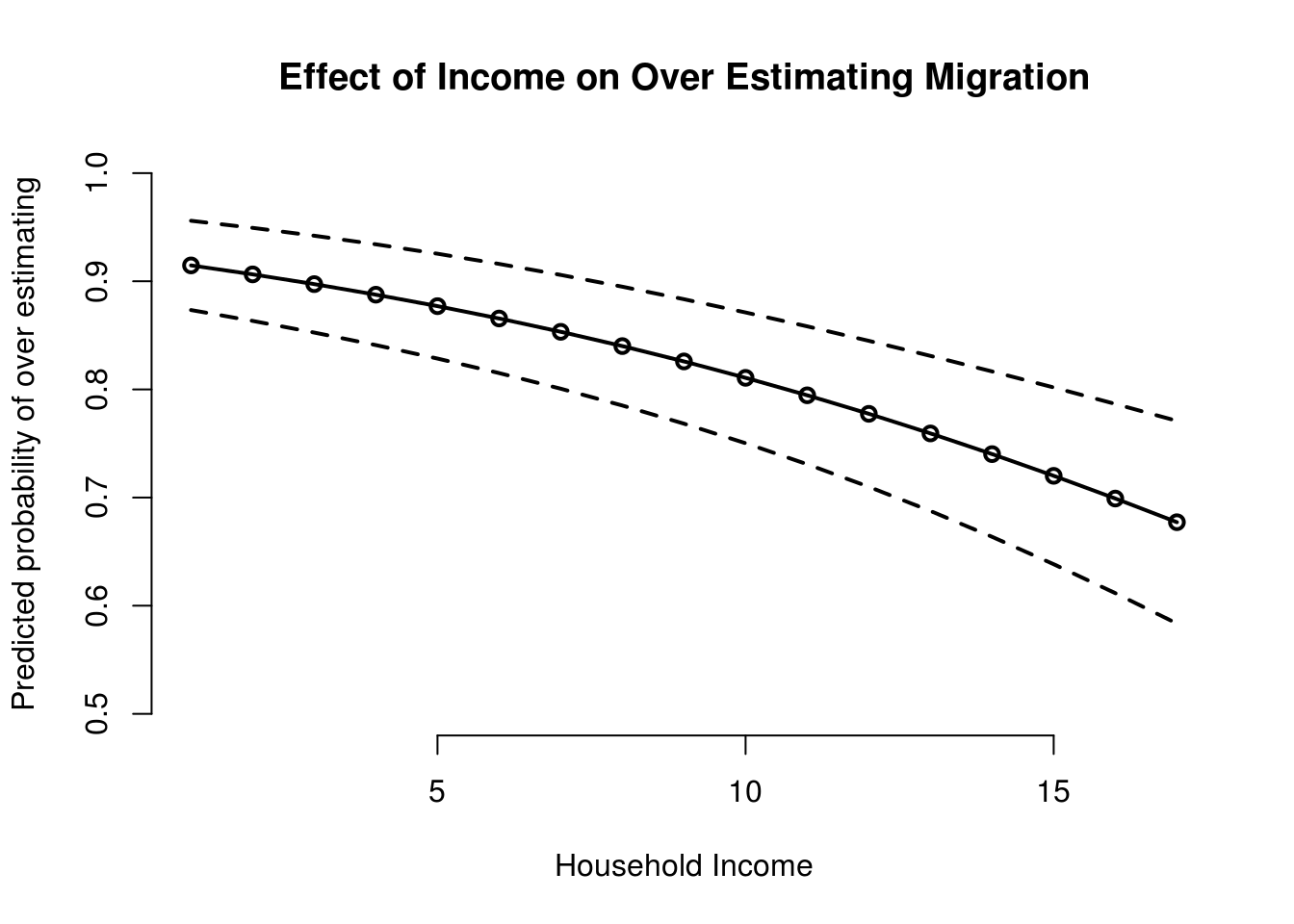
The plot indicates that the probability of over estimating decreases with higher income.