2 Descriptive Statistics
2.1 Seminar
Create a new script with the following lines at the top, and save it as seminar2.R
rm(list = ls())
setwd("~/PUBLG100")
2.1.1 Loading data
The first step in any data analysis project is to load the data into your software of choice. Data come in many different file formats such as .csv, .tab, .dta, etc. Today we will load a dataset which is stored in R’s native file format: .RData. The function to load data from this file format is called: load(). If you managed to set your working directory correctly just now (setwd("~/PUBLG100")), then you should just be able to run the line of code below.
load("non_western_foreingners.RData")The non-western foreingers data is about the subjective perception of immigrants from non-western countries.
Let’s check the codebook of our data.
| Variable | Description |
|---|---|
| IMMBRIT | Out of every 100 people in Britain, how many do you think are immigrants from non-western countries? |
| over.estimate | 1 if estimate is higher than 10.7%. |
| RSex | 1 = male, 2 = female |
| RAge | Age of respondent |
| Househld | Number of people living in respondent’s household |
| party identification | 1 = Conservatives, 2 = Labour, 3 = SNP, 4 = Greens, 5 = Ukip, 6 = BNP, 7 = other |
| paper | Do you normally read any daily morning newspaper 3+ times/week? |
| WWWhourspW | How many hours WWW per week? |
| religious | Do you regard yourself as belonging to any particular religion? |
| employMonths | How many mnths w. present employer? |
| urban | Population density, 4 categories (highest density is 4, lowest is 1) |
| health.good | How is your health in general for someone of your age? (0: bad, 1: fair, 2: fairly good, 3: good) |
| HHInc | Income bands for household, high number = high HH income |
We can look at the variable names in our data with the names() function.
names(fdata) [1] "IMMBRIT" "over.estimate" "RSex" "RAge"
[5] "Househld" "paper" "WWWhourspW" "religious"
[9] "employMonths" "urban" "health.good" "HHInc"
[13] "party_self" The dim() function can be used to find out the dimensions of the dataset (dimension 1 = rows, dimension 2 = columns).
dim(fdata)[1] 1049 13So, the dim() function tells us that we have data from 1049 respondents with 13 variables for each respondent.
Let’s take a quick peek at the first 10 observations to see what the dataset looks like. By default the head() function returns the first 6 rows, but let’s tell it to return the first 10 rows instead.
head(fdata, n = 10) IMMBRIT over.estimate RSex RAge Househld paper WWWhourspW religious
1 1 0 1 50 2 0 1 0
2 50 1 2 18 3 0 4 0
3 50 1 2 60 1 0 1 0
4 15 1 2 77 2 1 2 1
5 20 1 2 67 1 0 1 1
6 30 1 1 30 4 1 14 0
7 60 1 2 56 2 0 5 1
8 7 0 1 49 1 1 8 0
9 30 1 1 40 4 0 3 1
10 2 0 1 61 3 1 0 1
employMonths urban health.good HHInc party_self
1 72 4 1 13 2
2 72 4 2 3 7
3 456 3 3 9 7
4 72 1 3 8 7
5 72 3 3 9 7
6 72 1 2 9 7
7 180 1 2 13 3
8 156 4 2 14 7
9 264 2 2 11 3
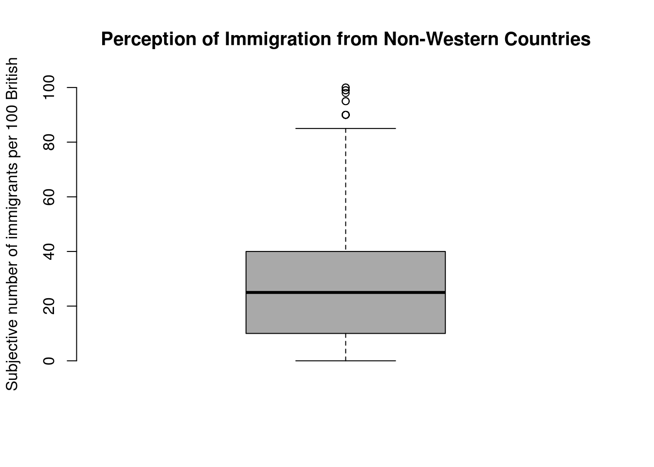
10 72 1 3 8 1We can visualize the data with the help of a boxplot, so let’s see how the perception of the number of immigrants is distributed.
# how good are we at guessing immigration
boxplot(
  fdata$IMMBRIT,
  main = "Perception of Immigration from Non-Western Countries",
  ylab = "Subjective number of immigrants per 100 British",
  frame.plot = FALSE, col = "darkgray"
  )
 Notice how the
 $ (dollar sign) is used to access the IMMBRIT variable from fdata. Our data is stored in what is called a data frame in R. We can think of a data frame as a table of rows and columns and similar to what most of us have seen as spreadsheets in programs like Microsoft Excel. Data frames can be created manually with the data.frame() function but are usually created by functions like read.csv() or read_excel() that load datasets from a file or from a web URL.
In the non-western foreignerns dataset, every column has a name and can be accessed using this $ (dollar sign) syntax. For example, household income can be accessed with fdata$HHInc.
2.1.2 Central Tendency
2.1.2.1 Arithmetic mean and median
The arithmetic mean (or average) is the most widely used measure of central tendency. We all know how to calculate the mean by dividing the sum of all observations by the number of observations. In R, we can get the sum with the sum() function:
sum(fdata$IMMBRIT)[1] 30453and the number of observations with the length() function:
length(fdata$IMMBRIT)[1] 1049So if we were interested in calculating the mean of the subjective proportion of immigrants in Britian (the true level at the time was 10.7), we could manually do the calculation of 30453/1049, but we can also combine these to functions in R in the following way:
sum(fdata$IMMBRIT) / length(fdata$IMMBRIT)[1] 29.03051R provides us with an even easier way to do the same with a function called mean(). Similarly, R also provides a median() function for finding the median. Now go ahead and calculate mean and median of IMMBRIT using those two functions.
immbrit_mean <- mean(fdata$IMMBRIT)
immbrit_mean
[1] 29.03051immbrit_median <- median(fdata$IMMBRIT)
immbrit_median[1] 252.1.2.2 Mode
There is no built-in function in base-R that returns the mode from a dataset. There are numerous packages that provide a mode function, but it’s quite simple to do it ourselves and it’s a good exercise for exploring some of R’s data manipulation functions.
We start by tabulating the data first and since our dataset is quite small, we can easily spot the mode with visual inspection. We will look at household income. The first row is the value of the variable and the second is its frequency in the data.
hhinc <- table(fdata$HHInc)
hhinc
  1   2   3   4   5   6   7   8   9  10  11  12  13  14  15  16  17
 19  47  50  55  61  73  55  33 212  43  48  32  66  49  38  39 129
The table() function tells us the number of respondents that fall into a household income band (the higher the value the richer the respondent). For example, 19 respondents are in income band 1, 47 fall into income band 2 and so on. The mode in this case is 9 which occurs 212 times.
But we’d really like to find the mode programmatically instead of manually scanning a long list of numbers. So let’s sort hhinc from largest to the smallest so we can pick out the mode. The sort() function allows us to do that with the decreasing = TRUE option.
sorted_hhinc <- sort(hhinc, decreasing = TRUE)
sorted_hhinc
  9  17   6  13   5   4   7   3  14  11   2  10  16  15   8  12   1
212 129  73  66  61  55  55  50  49  48  47  43  39  38  33  32  19
Because we sorted our list from largest to the smallest, the mode is the first element in the list.
hhinc_mode <- sorted_hhinc[1]
hhinc_mode
9
212 2.1.3 Factor Variables
Next, we want to find the maximum guess of the percentage of immigrants and we also want to see the party affiliation of the corresponding respondents. Our party affiliation variable party_self is a categorical variable. Each number (see codebook at the top) refers to a qualitative category. The numbers themselves don’t imply an ordering. In R, when categorical variables are stored as numeric data and if there are more than two distinct categories, we must convert them to factor variables to ensure that categorical data are handled correctly in functions that implement statistical models, tables and graphs.
We can convert categorical variables to factor variables using the factor() function. The factor() function needs the categorical variable and the distinct labels for each category (such as “Conservative”, “Labour”, “SNP” etc.) as the two arguments for creating factor variables.
fdata$party_self <- factor(fdata$party_self, labels = c("Tories", "Labour", "SNP", "Greens", "Ukip", "BNP", "other"))Let’s examine the new factor variable with a frequency table.
table(fdata$party_self)
Tories Labour    SNP Greens   Ukip    BNP  other
   284    280     16     23     31     32    383
Back to our original task: finding the party affiliation of those respondents who answered the maximum to the immigrant question. The max() function tells us the maximum value of IMMBRIT, and with the which() function, we identify the respondents who answered it. Notice, the double equal sign is a logical evaluation that can be true or false (check your cheat-sheet for other logical conditions). We can read the line with the which() function below as: in which observations (rows) in the data set is the value of the IMMBRIT variable equal to the maximum of the IMMBRIT variable.
max(fdata$IMMBRIT)[1] 100which(fdata$IMMBRIT == max(fdata$IMMBRIT))[1] 346 573Last week we learned that we can index datasets using the square brackets or the dollar sign. We can also combine the two. Below, we index the rows in square brackets and the column with the dollar sign.
imm_max_resp <- which(fdata$IMMBRIT == max(fdata$IMMBRIT))
party_imm_max_resp <- fdata[imm_max_resp, ]$party_self
party_imm_max_resp
[1] Labour Labour
Levels: Tories Labour SNP Greens Ukip BNP otherNow we know that the two respondents who think there is a 1:1 proportion of non-western immigrants to British people both self-identify with the Labour party.
2.1.4 Dispersion
While measures of central tendency represent the typical values for a dataset, we’re often interested in knowing how spread apart the values in the dataset are. The range is the simplest measure of dispersion as it tells us the difference between the highest and lowest values in a dataset. Let’s continue with the perception of immigration example and find out the range of our dataset using the range() and diff() functions.
Your turn, find the maximum and minimum of IMMBRIT using the range() function and get the range by taking the difference of minimum and maximum with the diff() function.
immi_range <- range(fdata$IMMBRIT)
diff(immi_range)
[1] 100Using a combination of range() and diff() functions we see that the difference between the two extremes (i.e. the highest and the lowest scores) in our dataset is 100.
2.1.4.1 Variance
Although the range gives us the difference between the two end points of the datasets, it still doesn’t quite give us a clear picture of the spread of the data. What we are really interested in is a measure that takes into account how far apart each immigration guess is from the mean. This is where the concept of variance comes in.
We can calculate the variance in R with the var() function. Take the variance of IMMBRIT.
var(fdata$IMMBRIT)[1] 443.66322.1.4.2 Standard Deviation
The standard deviation is simply the square root of the variance we calculated in the last section. We could manually take the square root of the variance to find the standard deviation, but R also provides a convenient sd() function.
Take the standard deviation of IMMBRIT.
sqrt(var(fdata$IMMBRIT)) # one way [1] 21.06331sd(fdata$IMMBRIT) # another way[1] 21.063312.1.4.3 Percentiles and Quantiles
The median value of a dataset is also known as the 50th percentile. It simply means that 50% of values are below the median and 50% are above it. In addition to the median, the 25th percentile (also known as the lower quartile) and 75th percentile (or the upper quartile) are commonly used to describe the distribution of values in a number of fields including standardized test scores, income and wealth statistics and healthcare measurements such as a baby’s birth weight or a child’s height compared to their respective peer group.
We can calculate percentiles using the quantile() function in R. For example, if we wanted to see the subjective number of immigrants in the 25th, 50th and 75th percentiles, we would call the quantile() function with c(0.25, 0.5, 0.75) as the second argument.
quantile(fdata$IMMBRIT, c(0.25, 0.5, 0.75))25% 50% 75%
10 25 40 The quantile() function tells us that 25% of respondents think the number is 10, 50% think the number is 25 or below and 75% think there are 40 or below immigrants per 100 British citizens.
2.1.5 Visualizing Data
Do people who self-identify with Ukip also think that there are more immigrants than people who identify with the Greens? To get a first idea, we can illustrate the subjective number of immigrants by party affiliation.
plot(fdata$IMMBRIT ~ fdata$party_self, las = 2, col = c("blue", "red", "yellow", "green", "purple", "brown", "gray"),
     frame.plot = FALSE, xlab = "", ylab = "Subj. # non-western immigrants per 100 British")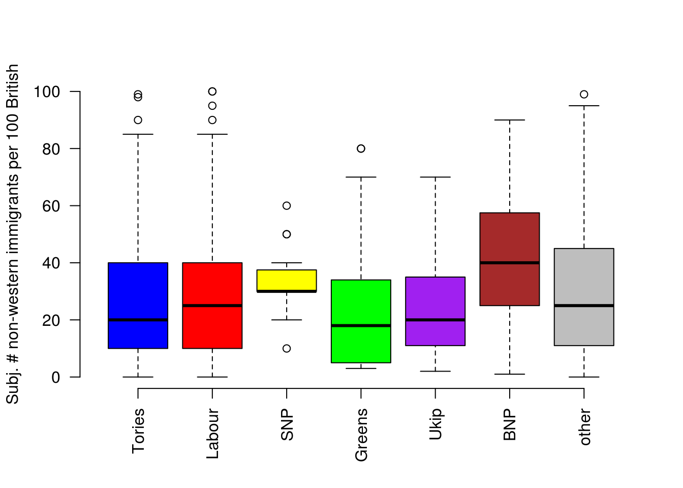
Now let’s see if we can visually examine the relationship between the number of months an employee has been with their employer and age using a scatter plot. Before we call the plot() function we need to reset the graphical parameters to make sure that our figure only contains a single plot by calling the par() function and using the mfrow=c(1,1) option.
plot(fdata$employMonths ~ fdata$RAge)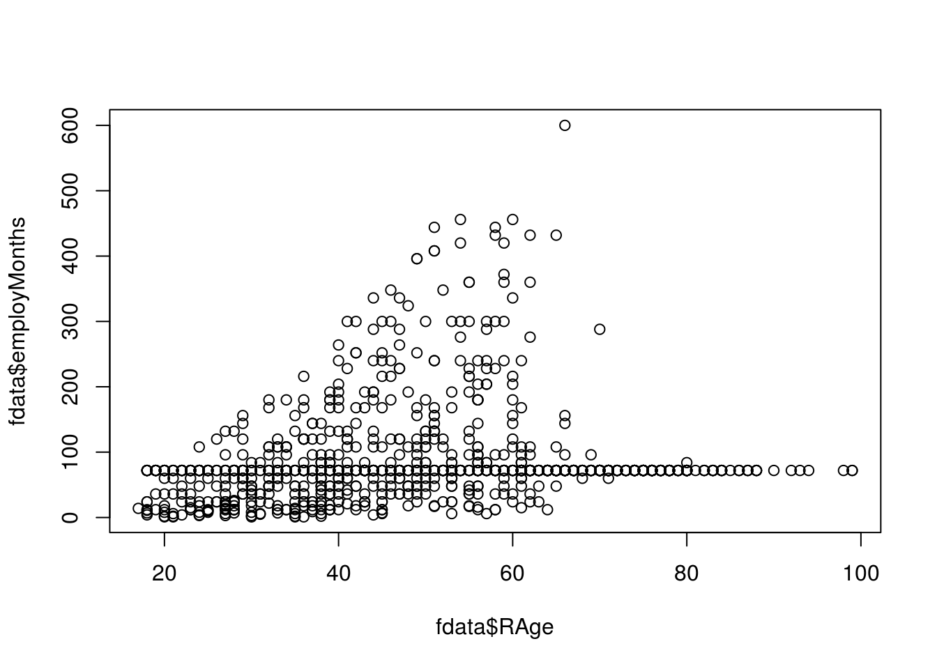
2.1.6 Additional Resources
2.1.7 Exercises
- Create a new file called “assignment2.R” in your
PUBLG100folder and write all the solutions in it. - Clear the workspace and set the working directory to your
PUBLG100folder. - Load the non-western foreigners dataset from your local drive into R.
- What is the level of measurement for each variable in the non-western foreigners dataset?
- Calculate the correct measure of central tendency for
RAge,Househld,religious. - Calculate the correct measure of dispersion for
RAge,Househld,religious. - How many respondents identify with the Greens?
- Calculate the variance and standard deviation of
IMMBRITfor each party affiliation. - Find the party affiliation of the oldest and youngest respondents.
- Find the 20th, 40th, 60th and 80th percentiles of
RAge. - Create a box plot for
IMMBRITgrouped by thepapervariable to show the difference betweenIMMBRITfor people who read daily morning newspapers three or more times per week and people who do not. - What is the mean of
IMMBRITfor men and for women? - What is the numerical difference between those two means?
- Save the script that includes all previous tasks.
- Source your script, i.e. run the entire script all at once without error message.