Throughout this module, we will make use of a number of packages from the “Tidyverse” — a collection of data science packages developed to make the management, manipulation, and visualization of data in R easier.1 We will begin by installing the Tidyverse and loading it for use:
1 Remember that “easier” is a relative term. Many of the things we will be doing would be harder were we to do them without using the Tidyverse packages, but they remain fiddly to implement in many cases.
library(tidyverse) ## This line needs to be run whenever you want to use the functions described on this page── Attaching core tidyverse packages ──────────────────────── tidyverse 2.0.0 ──
✔ dplyr 1.1.4 ✔ readr 2.1.5
✔ forcats 1.0.0 ✔ stringr 1.5.1
✔ ggplot2 3.5.1 ✔ tibble 3.2.1
✔ lubridate 1.9.4 ✔ tidyr 1.3.1
✔ purrr 1.0.2
── Conflicts ────────────────────────────────────────── tidyverse_conflicts() ──
✖ dplyr::filter() masks stats::filter()
✖ dplyr::lag() masks stats::lag()
ℹ Use the conflicted package (<http://conflicted.r-lib.org/>) to force all conflicts to become errorsFor the purposes of illustration, we will yse the mtcars dataset on this page. mtcars is a built-in dataset in R that contains information about 32 different car models. It includes 11 variables, such as fuel efficiency (mpg), engine size (disp), and the number of cylinders (cyl). This dataset is commonly used for teaching data manipulation, programming and visualisation because of its simplicity and variety of numeric and categorical variables. It is, on the other hand, very boring so my apologies for that.
%>% (The Pipe Operator)
The pipe operator %>% is one of the most important tools in the Tidyverse. It allows you to pass the output of one function directly into another, making your code cleaner and more readable.
Example:
dplyr
The dplyr package provides a range of functions for data manipulation. Below are some key functions you’ll use frequently:
filter()
Use filter() to subset rows based on conditions.
                mpg cyl  disp  hp drat    wt  qsec vs am gear carb
Datsun 710     22.8   4 108.0  93 3.85 2.320 18.61  1  1    4    1
Merc 240D      24.4   4 146.7  62 3.69 3.190 20.00  1  0    4    2
Merc 230       22.8   4 140.8  95 3.92 3.150 22.90  1  0    4    2
Fiat 128       32.4   4  78.7  66 4.08 2.200 19.47  1  1    4    1
Honda Civic    30.4   4  75.7  52 4.93 1.615 18.52  1  1    4    2
Toyota Corolla 33.9   4  71.1  65 4.22 1.835 19.90  1  1    4    1
Toyota Corona  21.5   4 120.1  97 3.70 2.465 20.01  1  0    3    1
Fiat X1-9      27.3   4  79.0  66 4.08 1.935 18.90  1  1    4    1
Porsche 914-2  26.0   4 120.3  91 4.43 2.140 16.70  0  1    5    2
Lotus Europa   30.4   4  95.1 113 3.77 1.513 16.90  1  1    5    2
Volvo 142E     21.4   4 121.0 109 4.11 2.780 18.60  1  1    4    2
select()
Use select() to choose specific columns.
                     mpg cyl gear
Mazda RX4           21.0   6    4
Mazda RX4 Wag       21.0   6    4
Datsun 710          22.8   4    4
Hornet 4 Drive      21.4   6    3
Hornet Sportabout   18.7   8    3
Valiant             18.1   6    3
Duster 360          14.3   8    3
Merc 240D           24.4   4    4
Merc 230            22.8   4    4
Merc 280            19.2   6    4
Merc 280C           17.8   6    4
Merc 450SE          16.4   8    3
Merc 450SL          17.3   8    3
Merc 450SLC         15.2   8    3
Cadillac Fleetwood  10.4   8    3
Lincoln Continental 10.4   8    3
Chrysler Imperial   14.7   8    3
Fiat 128            32.4   4    4
Honda Civic         30.4   4    4
Toyota Corolla      33.9   4    4
Toyota Corona       21.5   4    3
Dodge Challenger    15.5   8    3
AMC Javelin         15.2   8    3
Camaro Z28          13.3   8    3
Pontiac Firebird    19.2   8    3
Fiat X1-9           27.3   4    4
Porsche 914-2       26.0   4    5
Lotus Europa        30.4   4    5
Ford Pantera L      15.8   8    5
Ferrari Dino        19.7   6    5
Maserati Bora       15.0   8    5
Volvo 142E          21.4   4    4
group_by()
Group data by one or more variables for aggregation.
# A tibble: 32 × 11
# Groups:   cyl [3]
     mpg   cyl  disp    hp  drat    wt  qsec    vs    am  gear  carb
   <dbl> <dbl> <dbl> <dbl> <dbl> <dbl> <dbl> <dbl> <dbl> <dbl> <dbl>
 1  21       6  160    110  3.9   2.62  16.5     0     1     4     4
 2  21       6  160    110  3.9   2.88  17.0     0     1     4     4
 3  22.8     4  108     93  3.85  2.32  18.6     1     1     4     1
 4  21.4     6  258    110  3.08  3.22  19.4     1     0     3     1
 5  18.7     8  360    175  3.15  3.44  17.0     0     0     3     2
 6  18.1     6  225    105  2.76  3.46  20.2     1     0     3     1
 7  14.3     8  360    245  3.21  3.57  15.8     0     0     3     4
 8  24.4     4  147.    62  3.69  3.19  20       1     0     4     2
 9  22.8     4  141.    95  3.92  3.15  22.9     1     0     4     2
10  19.2     6  168.   123  3.92  3.44  18.3     1     0     4     4
# ℹ 22 more rows
summarise()
Summarize data using aggregate functions like mean(), sum(), or n().
mutate()
Add new columns or transform existing ones.
                     mpg cyl  disp  hp drat    wt  qsec vs am gear carb
Mazda RX4           21.0   6 160.0 110 3.90 2.620 16.46  0  1    4    4
Mazda RX4 Wag       21.0   6 160.0 110 3.90 2.875 17.02  0  1    4    4
Datsun 710          22.8   4 108.0  93 3.85 2.320 18.61  1  1    4    1
Hornet 4 Drive      21.4   6 258.0 110 3.08 3.215 19.44  1  0    3    1
Hornet Sportabout   18.7   8 360.0 175 3.15 3.440 17.02  0  0    3    2
Valiant             18.1   6 225.0 105 2.76 3.460 20.22  1  0    3    1
Duster 360          14.3   8 360.0 245 3.21 3.570 15.84  0  0    3    4
Merc 240D           24.4   4 146.7  62 3.69 3.190 20.00  1  0    4    2
Merc 230            22.8   4 140.8  95 3.92 3.150 22.90  1  0    4    2
Merc 280            19.2   6 167.6 123 3.92 3.440 18.30  1  0    4    4
Merc 280C           17.8   6 167.6 123 3.92 3.440 18.90  1  0    4    4
Merc 450SE          16.4   8 275.8 180 3.07 4.070 17.40  0  0    3    3
Merc 450SL          17.3   8 275.8 180 3.07 3.730 17.60  0  0    3    3
Merc 450SLC         15.2   8 275.8 180 3.07 3.780 18.00  0  0    3    3
Cadillac Fleetwood  10.4   8 472.0 205 2.93 5.250 17.98  0  0    3    4
Lincoln Continental 10.4   8 460.0 215 3.00 5.424 17.82  0  0    3    4
Chrysler Imperial   14.7   8 440.0 230 3.23 5.345 17.42  0  0    3    4
Fiat 128            32.4   4  78.7  66 4.08 2.200 19.47  1  1    4    1
Honda Civic         30.4   4  75.7  52 4.93 1.615 18.52  1  1    4    2
Toyota Corolla      33.9   4  71.1  65 4.22 1.835 19.90  1  1    4    1
Toyota Corona       21.5   4 120.1  97 3.70 2.465 20.01  1  0    3    1
Dodge Challenger    15.5   8 318.0 150 2.76 3.520 16.87  0  0    3    2
AMC Javelin         15.2   8 304.0 150 3.15 3.435 17.30  0  0    3    2
Camaro Z28          13.3   8 350.0 245 3.73 3.840 15.41  0  0    3    4
Pontiac Firebird    19.2   8 400.0 175 3.08 3.845 17.05  0  0    3    2
Fiat X1-9           27.3   4  79.0  66 4.08 1.935 18.90  1  1    4    1
Porsche 914-2       26.0   4 120.3  91 4.43 2.140 16.70  0  1    5    2
Lotus Europa        30.4   4  95.1 113 3.77 1.513 16.90  1  1    5    2
Ford Pantera L      15.8   8 351.0 264 4.22 3.170 14.50  0  1    5    4
Ferrari Dino        19.7   6 145.0 175 3.62 2.770 15.50  0  1    5    6
Maserati Bora       15.0   8 301.0 335 3.54 3.570 14.60  0  1    5    8
Volvo 142E          21.4   4 121.0 109 4.11 2.780 18.60  1  1    4    2
                    weight_kg
Mazda RX4           1188.4110
Mazda RX4 Wag       1304.0770
Datsun 710          1052.3334
Hornet 4 Drive      1458.2983
Hornet Sportabout   1560.3565
Valiant             1569.4283
Duster 360          1619.3234
Merc 240D           1446.9585
Merc 230            1428.8148
Merc 280            1560.3565
Merc 280C           1560.3565
Merc 450SE          1846.1194
Merc 450SL          1691.8982
Merc 450SLC         1714.5778
Cadillac Fleetwood  2381.3580
Lincoln Continental 2460.2830
Chrysler Imperial   2424.4492
Fiat 128             997.9024
Honda Civic          732.5511
Toyota Corolla       832.3413
Toyota Corona       1118.1043
Dodge Challenger    1596.6438
AMC Javelin         1558.0885
Camaro Z28          1741.7933
Pontiac Firebird    1744.0612
Fiat X1-9            877.7005
Porsche 914-2        970.6869
Lotus Europa         686.2847
Ford Pantera L      1437.8866
Ferrari Dino        1256.4498
Maserati Bora       1619.3234
Volvo 142E          1260.9858
pivot_longer() and pivot_wider()
Reshape data between long and wide formats.
# Example: pivot_longer
data <- tibble(id = 1:3, a = c(10, 20, 30), b = c(40, 50, 60))
data %>%
  pivot_longer(cols = a:b, names_to = "variable", values_to = "value")
# A tibble: 6 × 3
id variable value
<int> <chr> <dbl>
1 1 a 10
2 1 b 40
3 2 a 20
4 2 b 50
5 3 a 30
6 3 b 60# Example: pivot_wider
data_long <- tibble(id = c(1, 1, 2, 2), variable = c("a", "b", "a", "b"), value = c(10, 40, 20, 50))
data_long %>%
pivot_wider(names_from = variable, values_from = value)# A tibble: 2 × 3
id a b
<dbl> <dbl> <dbl>
1 1 10 40
2 2 20 50Joins
dplyr provides functions for combining datasets by matching rows. Common types of joins include:
full_join
Includes all rows from both datasets.
right_join
Includes all rows from the second dataset and matches from the first.
left_join
Includes all rows from the first dataset and matches from the second.
ggplot2
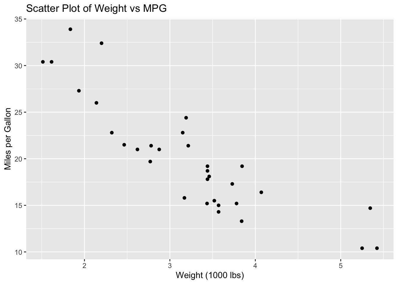
The ggplot2 package is the primary tool in the Tidyverse for data visualization. It allows you to create layered and customizable plots.
Example: Basic Scatter Plot
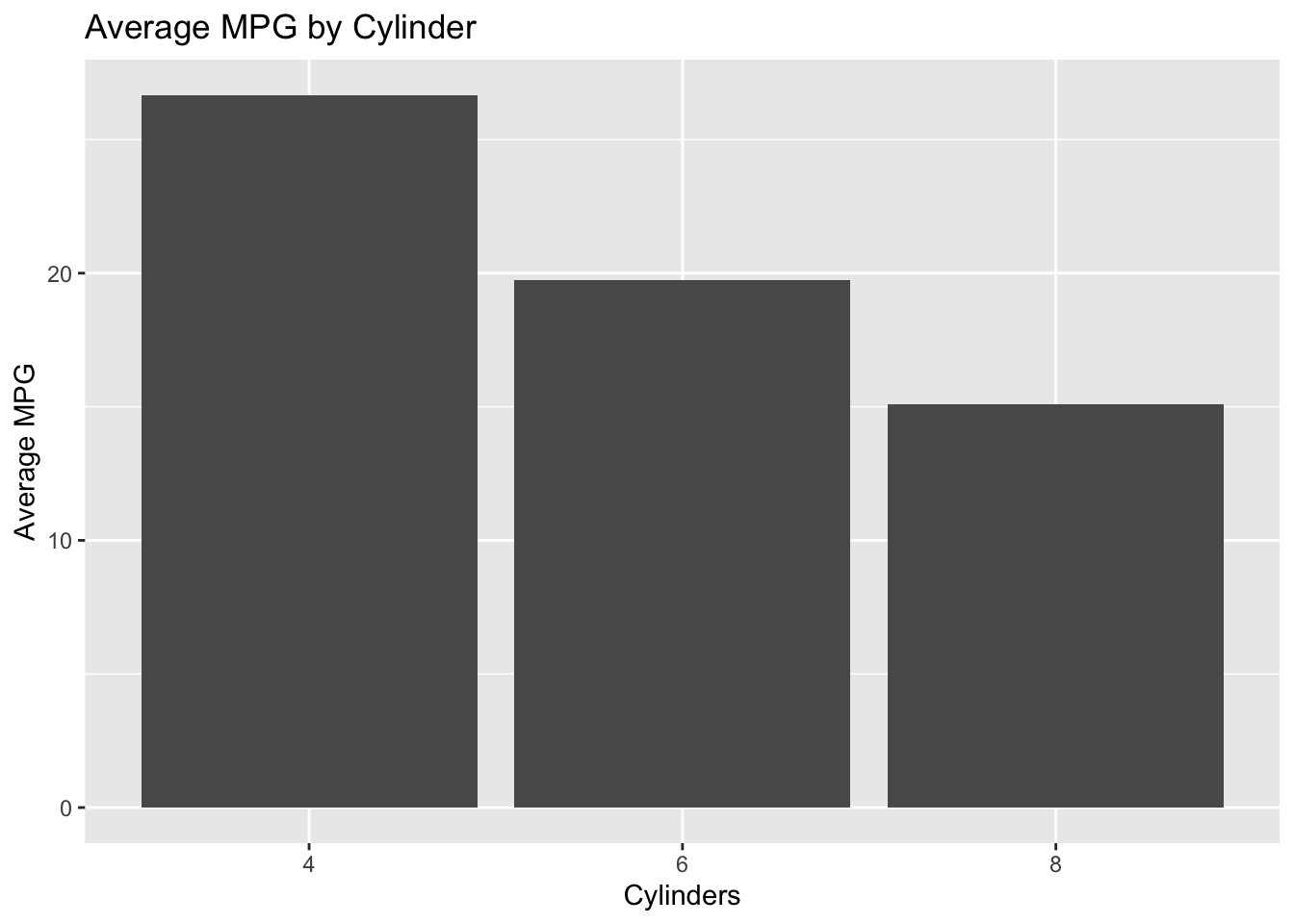
Example: Grouped Bar Plot
mtcars %>%
  group_by(cyl) %>%
  summarise(avg_mpg = mean(mpg)) %>%
  ggplot(aes(x = factor(cyl), y = avg_mpg)) +
  geom_bar(stat = "identity") +
  labs(title = "Average MPG by Cylinder",
       x = "Cylinders",
       y = "Average MPG")
This page is not a complete tutorial in the tidyverse! I will try to explain functions as we go along but if you wish to learn more about the Tidyverse, you may find the following resources helpful
Official Tidyverse Documentation
Tidyverse Packages Overview: https://www.tidyverse.org
A central hub for all Tidyverse packages, their documentation, and updates.dplyrDocumentation: https://dplyr.tidyverse.org
Learn more about data manipulation functions likefilter(),mutate(), andgroup_by().ggplot2Documentation: https://ggplot2.tidyverse.org
Explore the detailed reference for creating visualizations.
Books
R for Data Science by Hadley Wickham & Garrett Grolemund:
https://r4ds.had.co.nz
A free, comprehensive, and beginner-friendly guide to using the Tidyverse for data science.Tidyverse Skills for Data Science by Julia Silge:
Available via O’Reilly Learning. Focused on applied Tidyverse techniques.
Online Tutorials and Courses
Tidyverse on RStudio Cloud:
https://rstudio.cloud/learn/primers
Interactive primers that let you practice Tidyverse skills directly in your browser.DataCamp - Introduction to the Tidyverse:
https://www.datacamp.com/courses/intro-to-the-tidyverse
A hands-on course covering key Tidyverse packages.
Community and Forums
RStudio Community: https://community.rstudio.com
A helpful forum where you can ask questions and learn from other R users.Stack Overflow (R tag): https://stackoverflow.com/questions/tagged/r
A popular platform for troubleshooting R-related problems.
