2.1 Lecture slides
2.2 Analyzing the Preambles of Constitutions
Did the United States constitution influence the constitutions of other countries? There is a growing scholarly train of thought that suggests the influence of the US Constitution has decreased over time, as it is increasingly divergent from an increasing global consensus of the importance of human rights to constitutional settlements. However, there is a lack of empirical and systematic knowledge about the extent to which the U.S. Constitution impacts the revision and adoption of formal constitutions across the world.1
1 This problem set draws from material in Quantitative Social Science: An Introduction by Kosuke Imai.
David S. Law and Mila Versteeg (2012) investigate the influence of the US constitution empirically and show that other countries have, in recent decades, become increasingly unlikely to model the rights-related provisions of their own constitutions upon those found in the US Constitution. In this problem set, we will use some of the methods that we covered this week to replicate some parts of their analysis.
2.2.1 Packages
You will need to load the following packages before beginning the assignment
library(tidyverse)
library(quanteda)
# Run the following code if you cannot load the quanteda.textplots and quanteda.textstats packages
# devtools::install_github("quanteda/quanteda.textplots")
# devtools::install_github("quanteda/quanteda.textstats")

#run the following code if you cannot looad the css package
#install.packages("remotes")        # if you don't already have it
#remotes::install_github("kosukeimai/qss-package")

library(quanteda.textplots)
library(quanteda.textstats)
2.2.2 Data
We will use two sources of data for today’s assignment.
- Preambles of Constitutions –
constitutions.csv
This file contains the preambles of 155 (English-translated) constitutions. The data contains the following variables:
| Variable | Description |
|---|---|
country |
Name of the country |
continent |
Continent of the country |
year |
Year in which the constitution was written |
preamble |
Text of the preamble of the constitution |
Once you have downloaded this files and stored it somewhere sensible, you can load it into R using the following command:
You can take a quick look at the variables in the data by using the glimpse() function from the tidyverse package:
Rows: 155
Columns: 4
$ country   <chr> "afghanistan", "albania", "algeria", "andorra", "angola", "a…
$ continent <chr> "Asia", "Europe", "Africa", "Europe", "Africa", "Americas", …
$ year      <dbl> 2004, 1998, 1989, 1993, 2010, 1981, 1853, 1995, 1995, 1973, …
$ preamble  <chr> "In the name of Allah, the Most Beneficent, the Most Mercifu…
2.3 Tf-idf
- Explore the
constitutionsobject to get a sense of the data that we are working with. What is the average length of the texts stored in thepreamblesvariable?2 Which country has the longest preamble text?3 Which has the shortest?4 Has the average length of these preambles changed over time?5
2 The ntokens() function will be helpful here.
3 The which.max() function will be helpful here.
4 The which.min() function will be helpful here.
5 You will need to compare the length of the preambles variable to the year variable in some way (a good-looking plot would be nice!)
Reveal code
[1] 324.3097[1] "iran_islamic_republic_of"[1] "greece"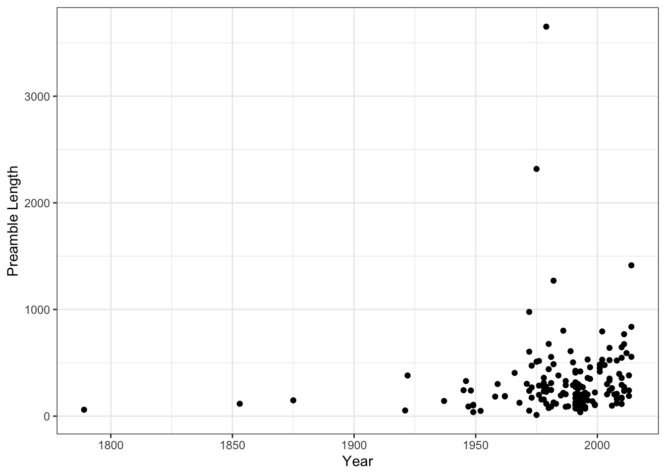
It is a little hard to tell whether there has been a systematic increase in preamble length across this time span because there are so few constitutions written in the earlier periods of the data. We can get a clearer view of the modern evolution of preamble length by focusing only on data since the 1950s:
`geom_smooth()` using method = 'loess' and formula = 'y ~ x'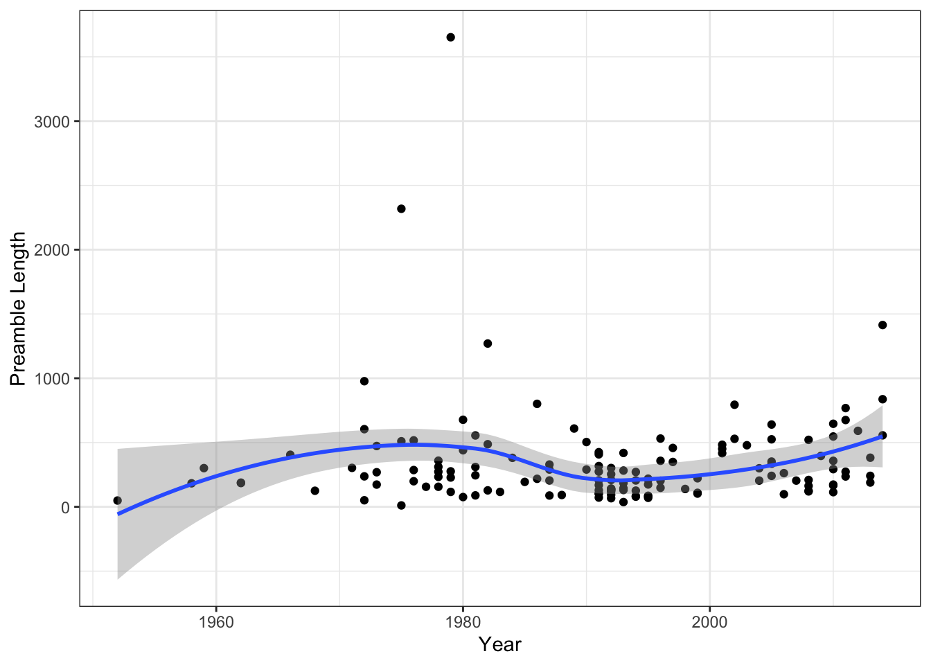
There is some evidence of an increase, though it is not a very clear trend.
- Convert the
constitutionsdata.frame into acorpus()object and then into adfm()object (remember that you will need to use thetokens()) function as well. Make some sensible feature selection decisions.
Reveal code
- Use the
topfeatures()function to find the most prevalent 10 features in the US constitution. Compare these features to the top features for three other countries of your choice. What do you notice?
Reveal code
      united    establish       states       people        order         form
           2            2            2            1            1            1
     justice      defense constitution      liberty
1 1 1 1 argentine justice nation general peace people god national
3 2 2 2 1 1 1 1
establish defense
1 1 man peoples dignity revolution full
4 3 3 3 3
revolutionary victory mart last human
3 3 3 2 2 peace committed agreement sudan constitution religious
4 3 3 3 2 2
shall governance agreements end
2 2 2 2 - Apply tf-idf weights to your dfm using the
dfm_tfidf()function. Repeat the exercise above using the new matrix. What do you notice?
Reveal code
     insure     america     perfect      states    domestic tranquility
   2.190332    1.889302    1.889302    1.870118    1.588272    1.588272
     ordain   establish     defense   blessings
1.412180 1.292527 1.236089 1.190332 argentine pre-existing constituting dwell congress provinces
6.570995 2.190332 2.190332 2.190332 1.889302 1.889302
compose object securing general
1.889302 1.889302 1.889302 1.870118 mart cuban jos cubans victory
6.570995 4.380663 4.380663 4.380663 4.035701
revolutionary peasants workers revolution last
3.446817 3.426421 3.176543 3.132611 2.824361 sudan agreement agreements 2005 conflict
5.667905 4.236541 3.426421 3.426421 3.426421
comprehensive end committed bestowed definitively
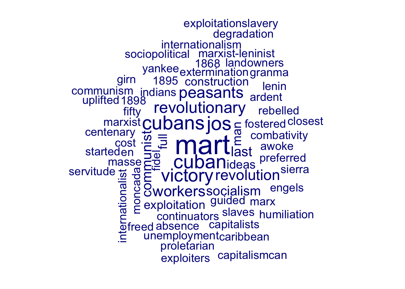
2.982723 2.380663 2.326075 2.190332 2.190332 - Make two word clouds for two for the USA and one other country using the
textplot_wordcloud()function. Marvel at how ugly these are.6
6 You may need to set the min_count argument to be a lower value than the default of 3 for the US constitution, as that text is very short.
2.4 Cosine Similarity
The cosine similarity (\(cos(\theta)\)) between two vectors \(\textbf{a}\) and \(\textbf{b}\) is defined as:
\[cos(\theta) = \frac{\mathbf{a} \cdot \mathbf{b}}{\left|\left| \mathbf{a} \right|\right| \left|\left| \mathbf{b} \right|\right|}\]
where \(\theta\) is the angle between the two vectors and \(\left| \mathbf{a} \right|\) and \(\left| \mathbf{b} \right|\) are the magnitudes of the vectors \(\mathbf{a}\) and \(\mathbf{b}\), respectively. In slightly more laborious, but possibly easier to understand, notation:
\[cos(\theta) = \frac{a_1b_1 + a_2b_2 + ... + a_Jb_J}{\sqrt{a_1^2 + a_2^2 + ... + a_J^2} \times \sqrt{b_1^2 + b_2^2 + ... + b_J^2}}\]
- Write a function that calculates the cosine similarity between two vectors.7
7 We can define a new function using the function() function. For example, if we want to calculate a new function for the mean, we can use mean_func <- function(x) sum(x)/length(x), where x is a vector.
Reveal code
cosine_sim <- function(a, b){

  # Calculate the inner product of the two vectors
  numerator <- sum(a * b)

  # Calculate the magnitude of the first vector
  magnitude_a <- sqrt(sum(a^2))

  # Calculate the magnitude of the second vector
  magnitude_b <- sqrt(sum(b^2))

  # Calculate the denominator
  denominator <- magnitude_a * magnitude_b

  # Calculate the similarity
  cos_sim <- numerator/denominator

  return(cos_sim)

}- Use the function you created above to calculate the cosine similarity between the preamble of the US and another country of your choice. Use the tf-idf version of your dfm for this question. Check that your function is working properly by comparing it to the cosine similarity calculated by the
textstat_simil()function.8
8 You can provide this function with an x vector and a y vector. You also need to specify method = "cosine" in order to calculate the cosine similarity, rather than some other metric of similarity.
Reveal code
[1] 0.02427221textstat_simil object; method = "cosine"
text149
text36 0.0243Great! Our function works.
- Use the
textstat_simil()function to calculate the cosine similarity between the preamble for the US constitution and all other preambles in the data.9 Assign the output of this function to the originalconstitutionsdata.frame using theas.numeric()function. Which 3 constitutions are most similar to the US? Which are the 3 least similar?10
9 You can also provide this function with an x matrix and a y vector. This will enable you to calculate the similarity between all rows in x and the vector used for y.
10 Use the order() function to achieve this.
Reveal code
# Calculate the cosine similarity
cosine_sim <- textstat_simil(x = constitutions_dfm_tf_idf,
                             y = constitutions_dfm_tf_idf[docvars(constitutions_dfm_tf_idf)$country == "united_states_of_america",],
                             method = "cosine")


# Assign variable to data.frame
constitutions$cosine_sim <- as.numeric(cosine_sim)

# Find the constitutions that are most and least similar
constitutions$country[order(constitutions$cosine_sim, decreasing = T)][1:3]
[1] "united_states_of_america" "argentina"
[3] "philippines" [1] "greece" "lithuania" "slovenia" - Calculate the average cosine similarity between the constitution of the US and the constitutions of other countries for each decade in the data for all constitutions written from the 1950s onwards.
There are a couple of coding nuances that you will need to tackle to complete this question.
First, you will need to convert the
yearvariable to adecadevariable. You can do this by using the%%“modulo” operator, which calculates the remainder after the division of two numeric variables. For instance,1986 %% 10will return a value of6. If you subtract that from the original year, you will be left with the correct decade (i.e.1986 - 6 = 1980).Second, you will need to calculate the decade-level averages of the cosine similarity variable that you created in answer to the question above. To do so, you should use the
group_by()andsummarise()functions.11group_by()allows you to specify the variable by which the summarisation should be applied, and thesummarise()function allows you to specify which type of summary you wish to use (i.e. here you should be using themean()function).
11 See this page if you have forgotten how these functions work.
Reveal code
- Create a line graph (
geom_line()in ggplot) with the averages that you calculated above on the y-axis and with the decades on the x-axis. Have constitution preambles become less similar to the preamble of the US constituion over recent history?
Reveal code
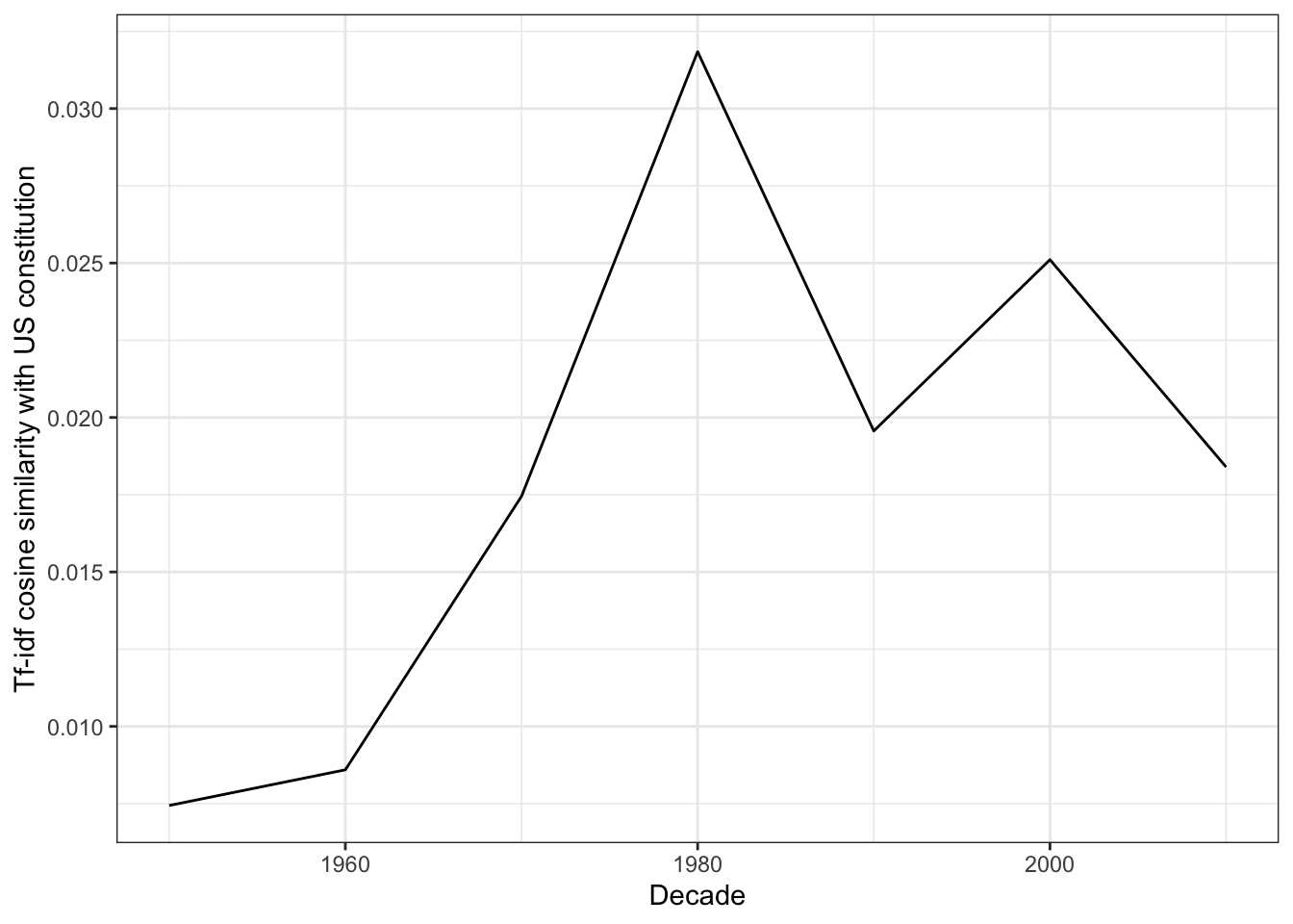
There is no clear evidence that constitutions are less similar to the US’s over time. This is contrary to the finding in Law and Versteeg (2012), but consistent with other work in the area. For instance, Elkins et. al., 2012 suggest that despite the addition of various “bells and whistles” in contemporary constitutions, “the influence of the U.S. Constitution remains evident.”
2.5 Fightin’ Words
Beyond calculating the similarity between constitutions, we might also be interested in describing the linguistic variation between constitutions in different parts of the world. To characterise these differences, we will make use of the Fightin’ Words method proposed by (Munroe, et. al, 2008).
Recall from the lecture that this method starts by calculating the probability of observing a given word for a given category of documents (here, departments):
\[\hat{\mu}_{j,k} = \frac{W^*_{j,k} + \alpha_0}{n_k + \sum_{j=1}^J + \alpha_0}\]
Where:
- \(W^*_{j,k}\) is the number of times feature \(j\) appears in documents in category \(k\)
- \(n_k\) is the total number of tokens in documents in category \(k\)
- \(\alpha_0\) is a “smoothing” parameter, which shrinks differences in common words towards 0
Next, we take the ratio of the log-odds for category \(k\) and \(k'\):
\[\text{log-odds-ratio}_{j,k} = log\left( \frac{\hat{\mu}_{j,k}}{1-\hat{\mu}_{j,k}}\right) - log\left( \frac{\hat{\mu}_{j,k'}}{1-\hat{\mu}_{j,k'}}\right) \]
Finally, we standardize the ratio by its variance (which again downweights differences in rarely-used words):
\[\text{Fightin' Words Score}_j = \frac{\text{log-odds-ratio}_{j,k}}{\sqrt{Var(\text{log-odds-ratio}_{j,k})}}\]
I have provided a function below which will calculate the Fightin’ Words scores for a pair of groups defined by any covariate in the data.
fightin_words <- function(dfm_input, covariate, group_1 = "Political Science", group_2 = "Economics", alpha_0 = 1){

  # Subset DFM
  fw_dfm <- dfm_subset(dfm_input, get(covariate) %in% c(group_1, group_2))
  fw_dfm <- dfm_group(fw_dfm, get(covariate))
  fw_dfm <- fw_dfm[,colSums(fw_dfm)!=0]
  dfm_input_trimmed <- dfm_match(dfm_input, featnames(fw_dfm))

  # Calculate word-specific priors
  alpha_w <- (colSums(dfm_input_trimmed))*(alpha_0/sum(dfm_input_trimmed))
  fw_dfm <- fw_dfm + alpha_w
  fw_dfm <- as.dfm(fw_dfm)
  mu <- fw_dfm %>% dfm_weight("prop")

  # Calculate log-odds ratio
  lo_g1 <- log(as.numeric(mu[group_1,])/(1-as.numeric(mu[group_1,])))
  lo_g2 <- log(as.numeric(mu[group_2,])/(1-as.numeric(mu[group_2,])))
  fw <- lo_g1 - lo_g2

  # Calculate variance
  fw_var <- as.numeric(1/(fw_dfm[1,])) + as.numeric(1/(fw_dfm[2,]))

  fw_scores <- data.frame(score = fw/sqrt(fw_var),
                          n = colSums(fw_dfm),
                          feature = featnames(fw_dfm))

  return(fw_scores)

}
There are 5 arguments to this function:
| Argument | Description |
|---|---|
| dfm_input | A dfm which measures word frequencies for each document |
| covariate | The name of a covariate (which should be entered as a string i.e. “covariate_name”) which contains the group labels (here, “continent”) |
| group_1 | The name of the first group |
| group_2 | The name of the second group |
| alpha_0 | The regularization parameter, which needs to be a positive integer |
The function returns a data.frame whose observations correspond to each feature used in the texts relating to the two groups and which contains three variables:
| Variable | Description |
|---|---|
feature |
The feature names |
fw |
The Fightin’ Words score for each feature |
n |
The number of times each feature is used across all documents of the two groups |
- Use the function above12 to calculate the Fightin’ Words scores that distinguish between constitutions of countries in Africa and Europe. What are the 10 words most strongly associated with each continent?
12 You will need to copy the code and paste it into your R script.
Reveal code
 [1] "political"  "unity"      "man"        "rights"     "power"
[6] "solemnly" "charter" "person" "december" "attachment" [1] "republic" "citizens" "responsibility"
[4] "state" "self-determination" "historical"
[7] "statehood" "centuries" "basic"
[10] "members" The words associated with African constitutions relate to rights, power and unity, while the words associated with European constitutions appear to relate more to responsibility, self-determination, and historical experiences.
- Create a graph which plots each of the feature names. The x-axis of the plot should be the log frequency of each term and the y-axis should be the Fightin’ Words score for the feature. Use the
cexandalphafunctions to scale the size and opacity of the words according to their Fightin’ Words scores.
Reveal code
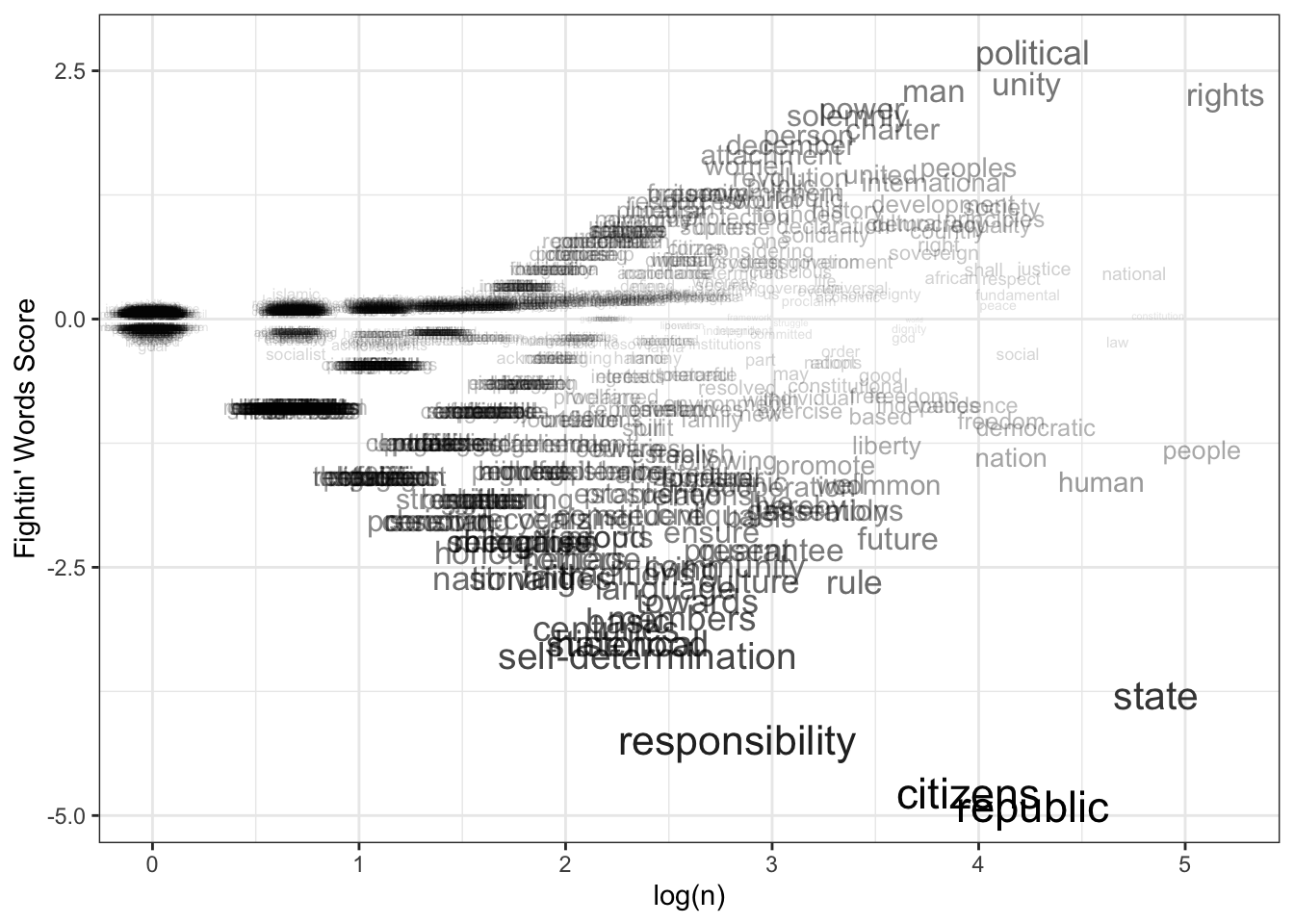
More effort, but isn’t that prettier than a word cloud?
2.6 Homework
In the lecture, we saw how we could use cosine similarity to find modules in UCL that are similar to PUBL0099. How effective was this strategy? In this homework, you will use the validation data that we generated in class to evaluate the cosine similarity measure.
Using the buttons above, you can download two datasets. The first, module_similarity_validation_data.csv, includes the results of the validation exercise that you all completed during the lecture. This data includes the following variables.
| Variable | Description |
|---|---|
code |
Module code |
prop_selected |
The proportion of times the module was selected as most similar to PUBL0099 in the pairwise comparisons in which it was included. |
Load this data using the following code:
The second homework data file – module_catalogue.Rdata – contains the full corpus of module descriptions. You can load this file and view the variables it contains by using the following code:
tibble [6,248 × 10] (S3: tbl_df/tbl/data.frame)
 $ teaching_department   : chr [1:6248] "Greek and Latin" "Greek and Latin" "Bartlett School of Sustainable Construction" "Bartlett School of Architecture" ...
 $ level                 : num [1:6248] 5 4 7 5 7 7 4 7 7 7 ...
 $ intended_teaching_term: chr [1:6248] "Term 1|Term 2" "Term 1" "Term 1" "Term 2" ...
 $ credit_value          : chr [1:6248] "15" "15" "15" "30" ...
 $ mode                  : chr [1:6248] "" "" "" "" ...
 $ subject               : chr [1:6248] "Ancient Greek|Ancient Languages and Cultures|Classics" "Ancient Greek|Ancient Languages and Cultures|Classics" "" "" ...
 $ keywords              : chr [1:6248] "ANCIENT GREEK|LANGUAGE" "ANCIENT GREEK|LANGUAGE" "Infrastructure finance|Financial modelling|Investment" "DESIGN PROJECT ARCHITECTURE" ...
 $ title                 : chr [1:6248] "Advanced Greek A (GREK0009)" "Greek for Beginners A (GREK0002)" "Infrastructure Finance (BCPM0016)" "Design Project (BARC0135)" ...
 $ module_description    : chr [1:6248] "Teaching Delivery: This module is taught in 20 bi-weekly lectures and 10 weekly PGTA-led seminars.\n\nContent: "| __truncated__ "Teaching Delivery: This module is taught in 20 bi-weekly lectures and 30 tri-weekly PGTA-led seminars.\n\nConte"| __truncated__ "This module offers a broad overview of infrastructure project development, finance, and investment. By explorin"| __truncated__ "Students take forward the unit themes, together with personal ideas and concepts from BARC0097, and develop the"| __truncated__ ...
$ code : chr [1:6248] "GREK0009" "GREK0002" "BCPM0016" "BARC0135" ...- Construct a dfm using the module descriptions stored in
modules$module_description. Weight the dfm using tf-idf weights.
Reveal code
- Calculate the cosine similarity between each document and the
module_descriptionfor PUBL0099.13
13 You will need to subset your dfm using an appropriate variable for the code variable.
Reveal code
- Merge these cosine similarity scores with the validation data.14 You may find it helpful to first create a new variable in the
modulesdata.frame that contains the cosine similarity scores.
14 You should use the full_join function to achieve this. This function takes two data.frames as the first and second argument. It also takes a by argument which should be set equal to the name of the variable that you are merging on (here, "code"). See the help file ?full_join if you are struggling.
Reveal code
- Create a plot which shows the association between the cosine similarity scores and the
prop_selectedvariable. You may first wish to exclude the PUBL0099 observation from the data. What does this plot suggest about the validity of the similarity metric?
Reveal code
`geom_smooth()` using method = 'gam' and formula = 'y ~ s(x, bs = "cs")'Warning: Removed 6167 rows containing non-finite outside the scale range
(`stat_smooth()`).Warning: Removed 6167 rows containing missing values or values outside the scale range
(`geom_point()`).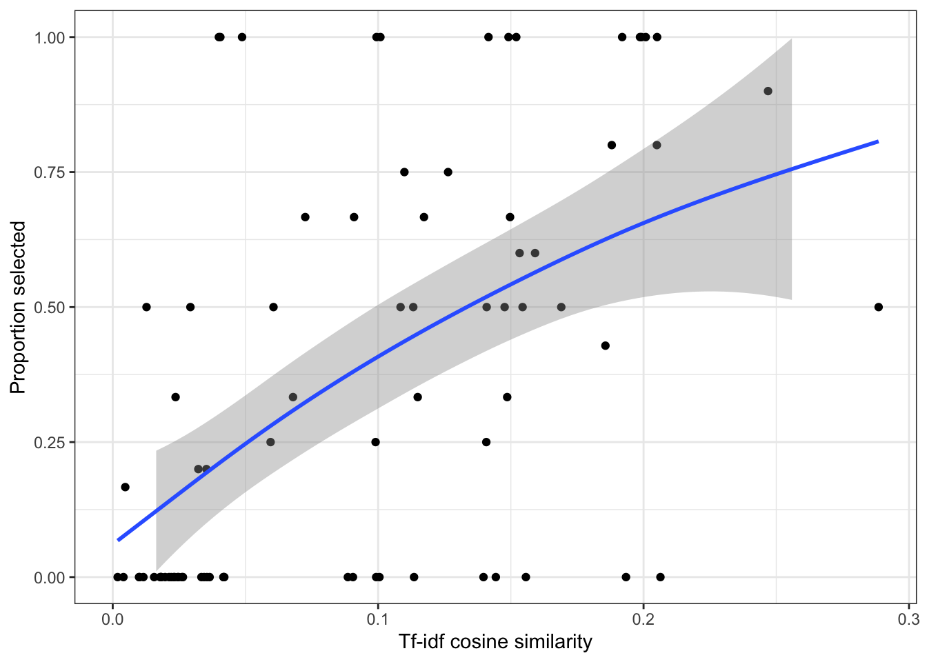
Looks good! There is a clear positive correlation between the similarity measure and the human generated outcome.
- Comment the
fightin_wordsfunction to explain what each line of code is doing in your own words.
# Fighting Words
fightin_words <- function(dfm_input, covariate, group_1 = "Political Science", group_2 = "Economics", alpha_0 = 1){

  # Inputs
  ## dfm_input: a document-feature matrix (dfm) from the quanteda package
  ## covariate: the name of a covariate (which should be entered as a string i.e. “covariate_name”) which contains the group labels (here, “continent”)
  ## group_1: the name of the first group (entered as a string)
  ## group_2: the name of the second group (entered as a string)
  ## alpha_0: the smoothing parameter, which needs to be a positive integer (default = 1)


  # Subset DFM
  fw_dfm <- dfm_subset(dfm_input, get(covariate) %in% c(group_1, group_2)) # subset to only the two groups of interest
  fw_dfm <- dfm_group(fw_dfm, get(covariate)) # group the dfm by the covariate (continent)
  fw_dfm <- fw_dfm[,colSums(fw_dfm)!=0] # remove tokens that never appear in either of the two groups
  dfm_input_trimmed <- dfm_match(dfm_input, featnames(fw_dfm)) # trim original dfm to match vocabulary of comparison dfm

  # Calculate word-specific priors
  alpha_w <- (colSums(dfm_input_trimmed))*(alpha_0/sum(dfm_input_trimmed)) # occurrence of each token in the full corpus * (smoothing parameter/ total tokens in corpus)
  fw_dfm <- fw_dfm + alpha_w # adds the feature-specific prior to dfm
  fw_dfm <- as.dfm(fw_dfm) # change back to dfm object
  mu <- fw_dfm %>% dfm_weight("prop") # calculate probabilities for each token in each group

  # Calculate log-odds ratio
  lo_g1 <- log(as.numeric(mu[group_1,])/(1-as.numeric(mu[group_1,]))) # log-odds for group 1
  lo_g2 <- log(as.numeric(mu[group_2,])/(1-as.numeric(mu[group_2,]))) # log-odds for group 2
  fw <- lo_g1 - lo_g2 # ratio in log-odds

  # Calculate variance
  fw_var <- as.numeric(1/(fw_dfm[1,])) + as.numeric(1/(fw_dfm[2,])) # variance formula

  fw_scores <- data.frame(score = fw/sqrt(fw_var), # final score
                          n = colSums(fw_dfm), # total counts
                          feature = featnames(fw_dfm)) # feature names

  return(fw_scores)

  # Outputs a dataframe with three columns:
  ## score: the fighting words score for each word
  ## n: the total count of each word across both groups
  ## feature: the word itself

}
Upload your the code, the plot, and the annotation to this Moodle page.

