4.1 Lecture slides
4.2 Topic Models of Human Rights Reports
The US State Department has produced regular reports on human rights practices across the world for many years. These monitoring reports play an important role both in the international human rights regime and in the production of human rights data. In a paper published in 2018, Benjamin Baozzi and Daniel Berliner analyse these reports in order to identify a set of topics and describe how these vary over time and space.
In today’s seminar, we will analyse the US State Department’s annual Country Reports on Human Rights Practices (1977–2012), by applying structural topic models (STMs) to identify the underlying topics of attention and scrutiny across the entire corpus and in each individual report. We will also assess the extent to which the prevalence of different topics in the corpus is related to covariates pertaining to each countries’ relationship with the US.
4.3 Packages
You will need to load the following packages before beginning the assignment
4.4 Data
Today we will use data on 4067 Human Rights Reports from the US State Department. The table below describes some of the variables included in the data:
| Variable | Description |
|---|---|
cname |
The name of the country which is the subject of the report |
year |
The year of the report |
report |
The text of the report (note that these texts have already been stemmed and stop words have been removed) |
alliance |
Whether the country has a formal military alliance with the United States (1) or not (0). |
p_polity2 |
The polity score for the country |
logus_aid_econ |
The (log) level of foreign aid provided to the country by the US. |
oecd |
OECD membership dummy |
civil_war |
Civil war dummy |
Once you have downloaded the file and stored it somewhere sensible, you can load it into R:
You can take a quick look at the variables in the data by using the glimpse() function from the tidyverse package:
Rows: 4,067
Columns: 16
$ cname             <chr> "Albania", "Albania", "Albania", "Albania", "Albania…
$ year              <dbl> 1980, 1981, 1982, 1983, 1984, 1985, 1986, 1987, 1988…
$ cowcode           <dbl> 339, 339, 339, 339, 339, 339, 339, 339, 339, 339, 33…
$ logwdi_gdpc       <dbl> 7.524573, 7.560410, 7.568337, 7.558117, 7.524482, 7.…
$ p_polity2         <dbl> -9, -9, -9, -9, -9, -9, -9, -9, -9, -9, 1, 1, 5, 5, …
$ alliance          <dbl> 0, 0, 0, 0, 0, 0, 0, 0, 0, 0, 0, 0, 0, 0, 0, 0, 0, 0…
$ logus_aid_econ    <dbl> 0.00000, 0.00000, 0.00000, 0.00000, 0.00000, 0.00000…
$ civilwar          <dbl> 0, 0, 0, 0, 0, 0, 0, 0, 0, 0, 0, 0, 0, 0, 0, 0, 0, 0…
$ oecd              <dbl> 0, 0, 0, 0, 0, 0, 0, 0, 0, 0, 0, 0, 0, 0, 0, 0, 0, 0…
$ logtrade_with_US  <dbl> 3.010621, 2.502255, 3.131137, 2.263844, 2.627563, 2.…
$ latentmean_Fariss <dbl> -0.915279270, -1.060029900, -1.053791400, -1.0242505…
$ gd_ptsa           <dbl> 3, 3, 3, 3, 3, 3, 3, 3, 3, 3, 3, 3, 2, 2, 3, 3, 3, 4…
$ years_to_election <dbl> 0, 3, 2, 1, 0, 3, 2, 1, 0, 3, 2, 1, 0, 3, 2, 1, 0, 3…
$ rep_pres          <dbl> 0, 1, 1, 1, 1, 1, 1, 1, 1, 1, 1, 1, 1, 0, 0, 0, 0, 0…
$ pres_chambers     <dbl> 2, 1, 1, 1, 1, 1, 1, 0, 0, 0, 0, 0, 0, 2, 2, 0, 0, 0…
$ report            <chr> "albania isol balkan nation peopl govern communist r…
4.5 STM without covariates
We will begin by implementing the null model of the Structural Topic Model. This model is equivalent to the Correlated Topic Model – a close cousin of the LDA model that we covered in the lecture, though one in which the topics in the corpus are allowed to be correlated with each other (LDA assumes that topics are uncorrelated).
The stm() function from the stm package can be used to fit the model. There are a few different arguments that you will need to specify for this function:
| Argument | Description |
|---|---|
documents |
The DFM on which you intend to fit the stm model. |
K |
The number of topics you wish to estimate. |
prevalence |
A formula (with no response variable) specifying the covariates you wish to use to model the topic prevalences across documents. |
content |
A formula (with no response variable) specifying the covariate you wish to use to model the content of each topic across documents. |
seed |
A seed number to make the results replicable. |
- Create a corpus from the
human_rightsdata. Then create a dfm, making some feature selection decisions.1
1 Topic models can take a long time to estimate so I would advise that you trim the DFM to keep it reasonably small for now.
Reveal code
- Use the
stm()function from thestmpackage to fit a topic model. Choose an appropriate number of topics. You should not use any covariates in answer to this question. As the STM model will take a while to run (probably a minute or two), you should make sure you save the output of the model so that you don’t need to run this code repeatedly.
Reveal code
- Use the
plot()function to assess how common each topic is in this corpus. What is the most common topic? What is the least common?
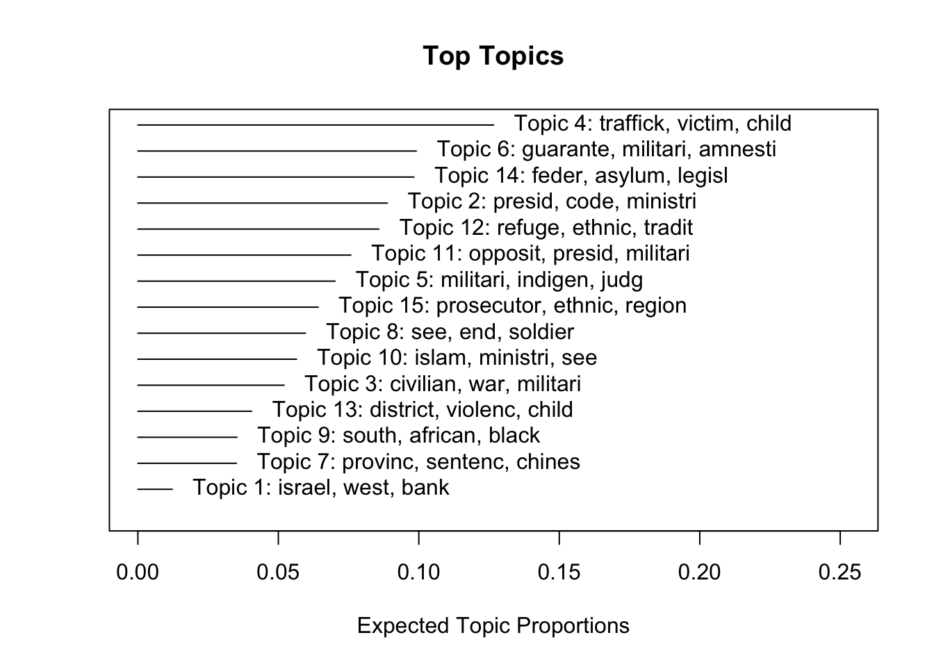
- Use the
labelTopics()function to extract the most distinctive words for each topic. Do some interpretation of these topic “labels”.2 Is there a sexual violence topic? Is there a topic about electoral manipulation? Create two word clouds illustrating two of the most interesting topics using thecloud()function.
2 Note that the stm package provides various different metrics for weighting words in estimated topic models. The most relevant two for our purposes are Highest Prob and FREX. Highest Prob simply reports the words that have the highest probability within each topic (i.e. inferred directly from the \(\beta\) parameters). FREX is a weighting that takes into account both frequency and exclusivity (words are upweighted when they are common in one topic but uncommon in other topics).
Reveal code
Topic 1 Top Words:
     Highest Prob: israel, west, bank, arab, territori, militari, occupi
     FREX: israel, west, bank, territori, arab, occupi, east
     Lift: israel, west, strip, arab, occupi, bank, territori
     Score: israel, arab, west, territori, jewish, bank, east
Topic 2 Top Words:
     Highest Prob: presid, code, ministri, minimum, enforc, minist, opposit
     FREX: code, franc, french, interior, minimum, radio, gendarmeri
     Lift: franc, gendarmeri, french, leagu, le, apprenticeship, slaveri
     Score: franc, gendarmeri, code, presid, french, ministri, disabl
Topic 3 Top Words:
     Highest Prob: civilian, war, militari, regim, attack, special, execut
     FREX: war, regim, iraq, southern, revolutionari, insurg, north
     Lift: iraq, revolutionari, regim, war, casualti, government-control, summarili
     Score: iraq, insurg, war, regim, revolutionari, civilian, militia
Topic 4 Top Words:
     Highest Prob: traffick, victim, child, sexual, violenc, ministri, ngos
     FREX: roma, sexual, traffick, societ, corrupt, exploit, victim
     Lift: roma, bisexu, transgend, chat, lesbian, reproduct, gay
     Score: roma, traffick, ngos, internet, sexual, child, ombudsman
Topic 5 Top Words:
     Highest Prob: militari, indigen, judg, ministri, crime, end, presid
     FREX: indigen, guerrilla, de, kidnap, paramilitari, congress, prosecutor
     Lift: guerrilla, jose, carlo, inter-american, san, homicid, el
     Score: guerrilla, indigen, jose, inter-american, carlo, ombudsman, el
Topic 6 Top Words:
     Highest Prob: guarante, militari, amnesti, recent, rate, will, peopl
     FREX: guarante, tion, ment, communist, now, growth, current
     Lift: vital, ment, tion, non-government, inter, guarante, invas
     Score: vital, tion, ment, communist, guarante, indian, now
Topic 7 Top Words:
     Highest Prob: provinc, sentenc, chines, detain, activist, china, provinci
     FREX: provinc, chines, china, provinci, dissid, activist, enterpris
     Lift: china, chines, provinc, dissid, anniversari, provinci, crackdown
     Score: china, chines, provinc, dissid, provinci, internet, communist
Topic 8 Top Words:
     Highest Prob: see, end, soldier, child, journalist, militari, civilian
     FREX: soldier, rebel, idp, fgm, girl, arm, unlik
     Lift: rebel, fgm, idp, loot, soldier, unlik, rob
     Score: rebel, idp, fgm, soldier, see, ngos, ethnic
Topic 9 Top Words:
     Highest Prob: south, african, black, end, parliament, africa, white
     FREX: black, african, south, white, africa, farm, magistr
     Lift: white, black, africa, african, color, south, customari
     Score: white, african, south, africa, black, parliament, magistr
Topic 10 Top Words:
     Highest Prob: islam, ministri, see, muslim, sentenc, council, sharia
     FREX: islam, sharia, non-muslim, king, muslim, bahai, christian
     Lift: bahai, non-muslim, sunni, sharia, moham, ali, islam
     Score: bahai, islam, sharia, sunni, non-muslim, king, arab
Topic 11 Top Words:
     Highest Prob: opposit, presid, militari, detain, minist, leader, detaine
     FREX: opposit, decre, coup, martial, ralli, ban, emerg
     Lift: martial, coup, campus, opposit, sedit, decre, lift
     Score: martial, opposit, coup, presid, decre, militari, presidenti
Topic 12 Top Words:
     Highest Prob: refuge, ethnic, tradit, presid, power, peopl, can
     FREX: king, loan, tradit, role, agricultur, known, citizenship
     Lift: loan, consensus, king, nonpolit, expatri, monarchi, modern
     Score: loan, king, ethnic, royal, tradit, dissid, refuge
Topic 13 Top Words:
     Highest Prob: district, violenc, child, see, death, end, muslim
     FREX: district, milit, tribal, custodi, bond, injur, villag
     Lift: milit, cast, tribal, ordin, epz, tribe, bond
     Score: milit, ngos, tribal, insurg, traffick, muslim, child
Topic 14 Top Words:
     Highest Prob: feder, asylum, legisl, immigr, parliament, equal, minor
     FREX: immigr, asylum, feder, applic, equal, racial, european
     Lift: kingdom, racist, racism, alien, german, treati, immigr
     Score: kingdom, parliament, feder, immigr, disabl, asylum, seeker
Topic 15 Top Words:
     Highest Prob: prosecutor, ethnic, region, presid, media, ministri, parliament
     FREX: prosecutor, russian, orthodox, registr, regist, soviet, region
     Lift: russian, russia, orthodox, soviet, jehovah, procur, psychiatr
Score: russian, orthodox, soviet, russia, parliament, ethnic, prosecutor 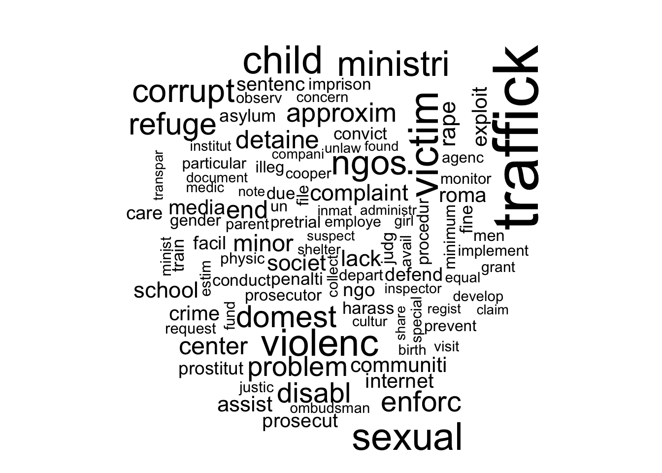

- Access the document-level topic-proportions from the estimated STM object (use
stm_out$theta). How many rows does this matrix have? How many columns? What do the rows and columns represent?
Reveal code
This matrix has 4067 rows and 15 columns. The rows here are the documents and the columns represent topics. The value for each cell of this matrix is the proportion of document \(d\) allocated to topic \(k\).
For example, let’s look at the first row of this matrix:
 [1] 0.0039523950 0.0042133431 0.1752261013 0.0002897973 0.0046490570
 [6] 0.6530379815 0.0840778178 0.0003162544 0.0012652509 0.0048260677
[11] 0.0110152909 0.0317211049 0.0016624187 0.0149808187 0.0087663007
We can see that the first document in our collection is mostly about topic 6, because 65% of the document is allocated to that topic.
- Pick one of the topics and plot it against the
yearvariable from thehuman_rightsdata. What does this plot suggest?
Reveal code
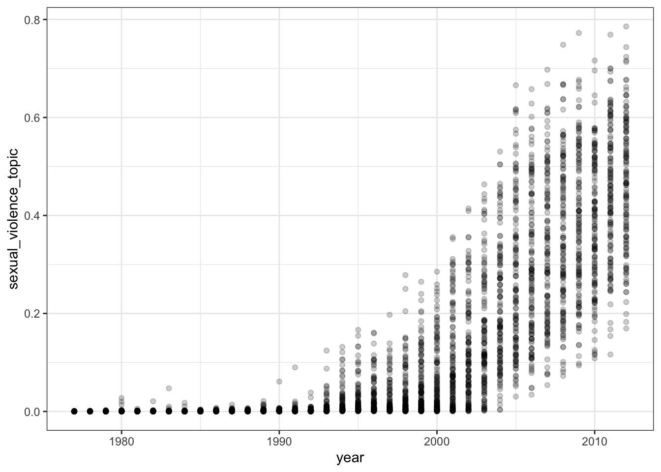
There is evidence that this topic has become much more prominent in the country reports over time.
4.6 STM with covariates
- A key innovation of the stm is that it allows us to include arbitrary covariates into the text model, allowing us to assess the degree to which topics vary with document metadata. In this question, you should fit another stm, this time including a covariate in the
prevalenceargument. You can pick any covariate that you think is likely to show interesting relationships with the estimated topics. Again, remember to save your model output so that you don’t need to estimate the model more than once.
Reveal code
- We will want to be able to keep track of the estimated topics from this model for use in the plotting functions later. Create a vector of topic labels from the words with the highest
"frex"scores for each topic.
Reveal code
[1] "israel_west_bank_territori_arab_occupi_east"
[2] "code_franc_french_minimum_interior_radio_extrajudici"
[3] "war_regim_iraq_southern_revolutionari_insurg_north"
[4] "roma_sexual_traffick_societ_corrupt_exploit_victim"
[5] "indigen_guerrilla_de_kidnap_paramilitari_congress_prosecutor"
[6] "guarante_tion_ment_communist_now_growth_current"
[7] "provinc_chines_china_provinci_dissid_activist_enterpris"
[8] "soldier_rebel_idp_fgm_girl_arm_unlik"
[9] "black_african_south_white_africa_farm_magistr"
[10] "islam_sharia_non-muslim_king_muslim_bahai_christian"
[11] "opposit_decre_coup_martial_ralli_ban_newspap"
[12] "king_loan_role_tradit_agricultur_known_citizenship"
[13] "district_milit_tribal_bond_custodi_injur_villag"
[14] "immigr_asylum_feder_applic_equal_racial_european"
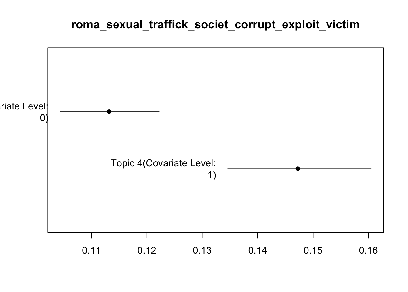
[15] "prosecutor_russian_orthodox_registr_regist_soviet_region" Note that the topics here differ somewhat from the topics we recovered using the stm without covariates. This is because here we have estimated a slightly different model, resulting in a slightly different distribution over words. This is one of the core weaknesses of topic models as the results are at least somewhat sensitive to model specification.
- Use the
estimateEffect()function to estimate differences in topic usage by one of the covariates in thehuman_rightsdata. This function takes three main arguments:
| Argument | Description |
|---|---|
formula |
A formula for the regression. Should be of the form c(1,2,3) ~ covariate_name, where the numbers on the left-hand side indicate the topics for which you would like to estimate effects. |
stmobj |
The model output from the stm() function. |
metadata |
A data.frame where the covariates are to be found. You can use docvars(my_dfm) for the dfm you used to estimate the original model. |
Reveal code
- Use the
summary()function to extract the estimated regression coefficients. For which topics do you find evidence of a significant relationship with the covariate you selected?
Reveal code
Call:
estimateEffect(formula = c(1:15) ~ alliance, stmobj = stm_out_prevalence,
    metadata = docvars(human_rights_dfm))


Topic 1:

Coefficients:
             Estimate Std. Error t value Pr(>|t|)
(Intercept)  0.018014   0.001535  11.739  < 2e-16 ***
alliance    -0.010863   0.002554  -4.253 2.16e-05 ***
---
Signif. codes:  0 '***' 0.001 '**' 0.01 '*' 0.05 '.' 0.1 ' ' 1


Topic 2:

Coefficients:
             Estimate Std. Error t value Pr(>|t|)
(Intercept)  0.088464   0.003031  29.182   <2e-16 ***
alliance    -0.011958   0.005530  -2.162   0.0307 *
---
Signif. codes:  0 '***' 0.001 '**' 0.01 '*' 0.05 '.' 0.1 ' ' 1


Topic 3:

Coefficients:
             Estimate Std. Error t value Pr(>|t|)
(Intercept)  0.062277   0.002563  24.303  < 2e-16 ***
alliance    -0.029942   0.004457  -6.719 2.09e-11 ***
---
Signif. codes:  0 '***' 0.001 '**' 0.01 '*' 0.05 '.' 0.1 ' ' 1


Topic 4:

Coefficients:
            Estimate Std. Error t value Pr(>|t|)
(Intercept) 0.113109   0.004461  25.356  < 2e-16 ***
alliance    0.034314   0.007992   4.293  1.8e-05 ***
---
Signif. codes:  0 '***' 0.001 '**' 0.01 '*' 0.05 '.' 0.1 ' ' 1


Topic 5:

Coefficients:
            Estimate Std. Error t value Pr(>|t|)
(Intercept) 0.012421   0.002691   4.616 4.03e-06 ***
alliance    0.185554   0.005944  31.218  < 2e-16 ***
---
Signif. codes:  0 '***' 0.001 '**' 0.01 '*' 0.05 '.' 0.1 ' ' 1


Topic 6:

Coefficients:
            Estimate Std. Error t value Pr(>|t|)
(Intercept) 0.081515   0.003665  22.243  < 2e-16 ***
alliance    0.044115   0.006689   6.596 4.78e-11 ***
---
Signif. codes:  0 '***' 0.001 '**' 0.01 '*' 0.05 '.' 0.1 ' ' 1


Topic 7:

Coefficients:
             Estimate Std. Error t value Pr(>|t|)
(Intercept)  0.041081   0.002387  17.210   <2e-16 ***
alliance    -0.008466   0.003995  -2.119   0.0341 *
---
Signif. codes:  0 '***' 0.001 '**' 0.01 '*' 0.05 '.' 0.1 ' ' 1


Topic 8:

Coefficients:
             Estimate Std. Error t value Pr(>|t|)
(Intercept)  0.078359   0.003186   24.59   <2e-16 ***
alliance    -0.059236   0.005231  -11.32   <2e-16 ***
---
Signif. codes:  0 '***' 0.001 '**' 0.01 '*' 0.05 '.' 0.1 ' ' 1


Topic 9:

Coefficients:
             Estimate Std. Error t value Pr(>|t|)
(Intercept)  0.045399   0.002326  19.516  < 2e-16 ***
alliance    -0.023675   0.003738  -6.334 2.65e-10 ***
---
Signif. codes:  0 '***' 0.001 '**' 0.01 '*' 0.05 '.' 0.1 ' ' 1


Topic 10:

Coefficients:
             Estimate Std. Error t value Pr(>|t|)
(Intercept)  0.076367   0.003208   23.80   <2e-16 ***
alliance    -0.056660   0.005144  -11.01   <2e-16 ***
---
Signif. codes:  0 '***' 0.001 '**' 0.01 '*' 0.05 '.' 0.1 ' ' 1


Topic 11:

Coefficients:
             Estimate Std. Error t value Pr(>|t|)
(Intercept)  0.077145   0.002698  28.595   <2e-16 ***
alliance    -0.007542   0.004602  -1.639    0.101
---
Signif. codes:  0 '***' 0.001 '**' 0.01 '*' 0.05 '.' 0.1 ' ' 1


Topic 12:

Coefficients:
             Estimate Std. Error t value Pr(>|t|)
(Intercept)  0.103965   0.002956   35.17   <2e-16 ***
alliance    -0.073486   0.004845  -15.17   <2e-16 ***
---
Signif. codes:  0 '***' 0.001 '**' 0.01 '*' 0.05 '.' 0.1 ' ' 1


Topic 13:

Coefficients:
             Estimate Std. Error t value Pr(>|t|)
(Intercept)  0.049324   0.002583  19.096  < 2e-16 ***
alliance    -0.016406   0.004569  -3.591 0.000334 ***
---
Signif. codes:  0 '***' 0.001 '**' 0.01 '*' 0.05 '.' 0.1 ' ' 1


Topic 14:

Coefficients:
            Estimate Std. Error t value Pr(>|t|)
(Intercept) 0.071055   0.003512   20.23   <2e-16 ***
alliance    0.077002   0.006412   12.01   <2e-16 ***
---
Signif. codes:  0 '***' 0.001 '**' 0.01 '*' 0.05 '.' 0.1 ' ' 1


Topic 15:

Coefficients:
             Estimate Std. Error t value Pr(>|t|)
(Intercept)  0.081439   0.003383  24.070  < 2e-16 ***
alliance    -0.042845   0.006304  -6.796 1.23e-11 ***
---
Signif. codes:  0 '***' 0.001 '**' 0.01 '*' 0.05 '.' 0.1 ' ' 1
Most of them!
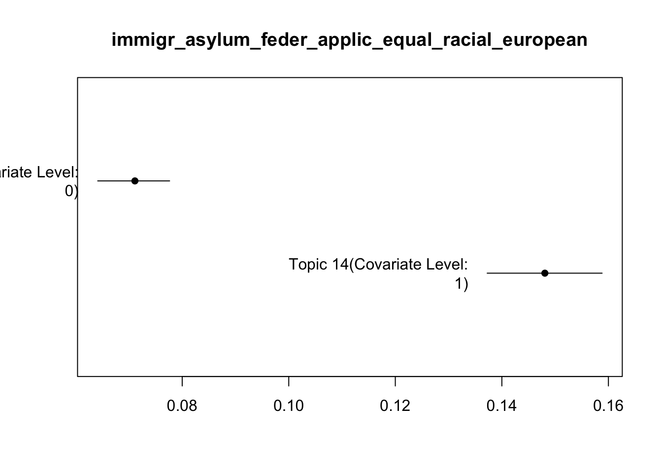
- Plot some of the more interesting differences that you just estimated using the
plot.estimateEffect()function. There are various different arguments that you can provide to this function. See the help file for assistance here (?plot.estimateEffect).
4.7 Homework
For the homework this week, you have three tasks. First, report findings from the model you ran above by producing a graph that demonstrates differences in topic prevalence by some covariate (i.e. not just the effect that I demonstrated in the plots above).
Second, fit an STM model which allows the content of the topics to vary by one of the covariates in the data. You can do so by making use of the content argument to the stm() function (see the lecture slides for an example). Once you have estimated the model, inspect the output and create at least one plot which demonstrates how word use for a given topic differs for the covariate you included in the model.
Third and should help you in grasping important equations fully. So please make sure to go through this carefully.
\[P(W_A|\mu_{\text{Comp+Genet}}) = \frac{M_A!}{\prod_{j=1}^J W_{A,j}!} \prod_{j=1}^J \mu_{\text{Comp+Genet},j}^{W_{A,j}} = 0.00121089\] Part A: First, tell me which equation this is. Where have we encountered this equation in the last week? What role does it for supervised and unsupervised techniques?
Part B: Now, show me how you’d reach the answer 0.00121089 by calculating this equation step-by-step in R.
Your task: Calculate each component of the equation manually in R (tip check slides week 3):
Calculate \(\mu_{\text{Comp+Genet},j}\) for each word \(j\) (the equal mixture)
Calculate \(M_A\) (total words in document)
Calculate the numerator: \(M_A!\)
Calculate the denominator: \(\prod_{j=1}^J W_{A,j}!\)
Calculate the product term: \(\prod_{j=1}^J \mu_{\text{Comp+Genet},j}^{W_{A,j}}\)
Combine them to get the final probability
Show your R code for each step and verify you get 0.00121089.
Use the following data:
# Word counts for Document A
word_counts_A <- c(
  gene = 2,
  dna = 3,
  genetic = 1,
  data = 3,
  number = 2,
  computer = 1
)


# Topic 1: Computer Science word probabilities
mu_comp <- c(
  gene = 0.02,
  dna = 0.01,
  genetic = 0.02,
  data = 0.30,
  number = 0.40,
  computer = 0.25
)


# Topic 2: Genetics word probabilities
mu_genet <- c(
  gene = 0.40,
  dna = 0.25,
  genetic = 0.30,
  data = 0.02,
  number = 0.02,
  computer = 0.01
)

# Step 1: Calculate μ_Comp+Genet for each word (equal mixture: 50-50)
# The mixture is equal: 50% Computer Science + 50% Genetics

mu_mixed <- _____ * mu_comp + _____ * mu_genet

# Step 2: Calculate M_A (total words in document)
M_A <- _____

# Step 3: Calculate the numerator: M_A!
# Hint: check function factorial() to check it type ?factorial
numerator <- _____

# Step 4: Calculate the denominator: ∏(W_{A,j}!)
# Hint: check function prod() to check it type ?prod

denominator <- _____

# Step 5: Calculate the product term: ∏(μ^W_{A,j})
product_term <- _____

# Step 6: Combine to get final probability
prob_A_mixed <- _____

# Check your answer
cat("Your answer:", prob_A_mixed, "\n")
cat("Expected:   0.00121089\n")
Upload your code and plots to this Moodle page, with a short description of the analysis that you implemented.