1 Representing Text As Data (I): Bag-of-Words – PUBL0099: Quantitative Text Analysis for Social Science

1.1 Lecture slides

1.2 Introduction

This seminar is designed to get you working with the quanteda package and some other associated packages. The focus will be on exploring the package, getting some texts into the corpus object format, learning how to convert texts into document-feature matrices, performing descriptive analyses on this data, and constructing and validating some dictionaries.

If you did not take PUBL0055 last term, or if are struggling to remember R from all the way back in December, then you should work through the exercises on the R refresher page before completing this assignment.

1.3 Measuring Moral Sentiment

Moral Foundations Theory is a social psychological theory that suggests that people’s moral reasoning is based on five separate moral values. These foundations, described in the table below, are care/harm, fairness/cheating, loyalty/betrayal, authority/subversion, and sanctity/degradation. According to the theory, people rely on these values to make moral judgments about different issues and situations. The theory also suggests that people differ in the importance they place on each of these values, and that these differences can help explain cultural and individual differences in moral judgment.¹ The table below gives a brief overview of these foundations:

¹ Moral Foundations Theory was developed and popularised by Jonathan Haidt and his coauthors. For a good and accessible introduction, see Haidt’s book on the topic.

Moral Foundations Theory categories.
Foundation	Description
Care	Concern for caring behaviour, kindness, compassion
Fairness	Concern for fairness, justice, trustworthiness
Authority	Concern for obedience and deference to figures of authority (religious, state, etc)
Loyalty	Concern for loyalty, patriotism, self-sacrifice
Sanctity	Concern for temperance, chastity, piety, cleanliness

Can we detect the use of these moral foundations from written text? Moral framing and rhetoric play an important role in political argument and entrenched moral divisions are frequently cited as the root cause of political polarization, particularly in online settings. Before we can answer important research questions such as whether there are large political differences in the use of moral language (as here, for example), or whether moral argument can reduce political polarization (as here, for example), we need to be able to measure the use of moral language at scale. In this seminar, we will therefore use a simple dictionary analysis to measure the degree to which a set of online texts display the types of moral language described by Moral Foundations Theory.

1.3.1 Data

We will use two sources of data for today’s assignment.

Moral Foundations Dictionary – mft_dictionary.csv
- This file contains lists of words that are thought to indicate the presence of different moral concerns in text. The dictionary was originally developed by Jesse Graham and Jonathan Haidt and is described in more detail in this paper.
- The file includes 5 categories of moral concern – authority, loyalty, santity, fairness, and care – each of which is associated with a different list of words
Moral Foundations Reddit Corpus – mft_texts.csv
- This file contains 17886 English Reddit comments that have been curated from 11 distinct subreddits. In addition to the texts – which cover a wide variety of different topics – the data also includes hand-annotations by trained annotators for the different categories of moral concern described by Moral Foundations Theory.

Once you have downloaded these files and stored them somewhere sensible, you can load them into R using the following commands:

mft_dictionary_words <- read_csv("mft_dictionary.csv")
mft_texts <- read_csv("mft_texts.csv")

1.3.2 Packages

You will need to install and load the following packages before beginning the assignment.

Run the following lines of code to install the following packages. Note that you only need to install packages once on your machine. One they are installed, you can delete these lines of code.

install.packages("tidyverse") # Set of packages helpful for data manipulation
install.packages("quanteda") # Main quanteda package
install.packages("quanteda.textplots") # Package with helpful plotting functions
install.packages("quanteda.textstats") # Package with helpful statistical functions
install.packages("remotes") # Package for installing other packages
remotes::install_github("kbenoit/quanteda.dictionaries")

With these packages installed onto your computer, you now need to load them so that the functions stored in the packages are available to you in this R session. You will need to run the following lines each time you want to use functions from these packages.

library(tidyverse)
library(quanteda)
library(quanteda.textplots)
library(quanteda.textstats)
library(quanteda.dictionaries)

1.4 Creating a corpus

1.4.1 Getting Help

Coding in R can be a frustrating experience. Fortunately, there are many ways of finding help when you are stuck.

The website http://quanteda.io has extensive documentation.
You can view the help file for any function by typing ?function_name
You can use example() function for any function in the package, to run the examples and see how the function works.

For example, to read the help file for the corpus() function you could use the following code.

Reveal code

?corpus

1.4.2 Making a corpus and corpus structure

A corpus object is the foundation for all the analysis we will be doing in quanteda. The first thing to do when you load some text data into R is to convert it using the corpus() function.

The simplest way to create a corpus is to use a set of texts already present in R’s global environment. In our case, we previously loaded the mft_texts.csv file and stored it as the mft_texts object. Let’s have a look at this object to see what it contains. Use the head() function applied to the mft_texts object and report the output. Which variable includes the texts of the Reddit comments?

Reveal code

head(mft_texts)

# A tibble: 6 × 9
   ...1 text       subreddit care  authority loyalty sanctity fairness non_moral
  <dbl> <chr>      <chr>     <lgl> <lgl>     <lgl>   <lgl>    <lgl>    <lgl>    
1     1 Alternati… worldnews FALSE FALSE     FALSE   FALSE    FALSE    TRUE     
2     2 Dr. Rober… politics  FALSE TRUE      FALSE   FALSE    FALSE    TRUE     
3     3 If you pr… worldnews FALSE FALSE     FALSE   FALSE    FALSE    TRUE     
4     4 Ben Judah… geopolit… FALSE TRUE      FALSE   FALSE    TRUE     FALSE    
5     5 Ergo, he … neoliber… FALSE FALSE     TRUE    FALSE    FALSE    TRUE     
6     6 He looks … nostalgia FALSE FALSE     FALSE   FALSE    FALSE    TRUE

The output tells us that this is a “tibble” (which is just a special type of data.frame) and we can see the first six lines of the data. The column labelled text contains the texts of the Reddit comments.

Use the corpus() function on this set of texts to create a new corpus. The first argument to corpus() should be the mft_texts object. You will also need to set the text_field to be equal to "text" so that quanteda knows that the text we are interested in is saved in that variable.

Reveal code

mft_corpus <- corpus(mft_texts, text_field = "text")

Once you have constructed this corpus, use the summary() method to see a brief description of the corpus. Which is the funniest subreddit name?

Reveal code

summary(mft_corpus)

Corpus consisting of 17886 documents, showing 100 documents:

    Text Types Tokens Sentences ...1           subreddit  care authority
   text1    67    101         7    1           worldnews FALSE     FALSE
   text2    59     72         2    2            politics FALSE      TRUE
   text3    81    177         3    3           worldnews FALSE     FALSE
   text4    65     82         5    4         geopolitics FALSE      TRUE
   text5    22     22         2    5          neoliberal FALSE     FALSE
   text6    21     28         2    6           nostalgia FALSE     FALSE
   text7    22     24         3    7           worldnews  TRUE     FALSE
   text8    41     44         3    8 relationship_advice  TRUE     FALSE
   text9    20     21         1    9       AmItheAsshole FALSE      TRUE
  text10    12     12         2   10            antiwork FALSE     FALSE
  text11    35     43         3   11              europe FALSE     FALSE
  text12    35     40         2   12          confession FALSE     FALSE
  text13    38     43         2   13 relationship_advice  TRUE     FALSE
  text14    46     62         2   14           worldnews  TRUE     FALSE
  text15    57     88         4   15            antiwork FALSE     FALSE
  text16    16     17         1   16           worldnews FALSE     FALSE
  text17    21     22         3   17       AmItheAsshole  TRUE     FALSE
  text18    20     21         3   18          neoliberal FALSE      TRUE
  text19    22     24         1   19            politics FALSE      TRUE
  text20    19     21         3   20          confession FALSE     FALSE
  text21    48     58         1   21            antiwork  TRUE     FALSE
  text22    78    115         4   22            politics FALSE     FALSE
  text23    12     13         1   23        Conservative FALSE     FALSE
  text24    38     66         1   24            antiwork FALSE     FALSE
  text25    18     26         2   25          confession FALSE     FALSE
  text26    22     32         1   26            politics FALSE     FALSE
  text27    70    103         7   27       AmItheAsshole  TRUE     FALSE
  text28    66     92         5   28           worldnews FALSE     FALSE
  text29    43     57         3   29          confession FALSE     FALSE
  text30    35     42         3   30       AmItheAsshole FALSE     FALSE
  text31    44     52         3   31           worldnews  TRUE     FALSE
  text32    31     39         4   32            antiwork FALSE     FALSE
  text33    20     24         2   33            antiwork  TRUE     FALSE
  text34    33     39         2   34            antiwork FALSE      TRUE
  text35    19     24         1   35          confession FALSE     FALSE
  text36    11     14         1   36        Conservative FALSE     FALSE
  text37    21     24         2   37           worldnews FALSE     FALSE
  text38    73    104         6   38 relationship_advice  TRUE      TRUE
  text39    32     41         3   39            antiwork FALSE     FALSE
  text40    73     95         2   40          neoliberal FALSE     FALSE
  text41    27     29         2   41        Conservative FALSE     FALSE
  text42    11     13         1   42            politics FALSE     FALSE
  text43    37     48         2   43              europe FALSE     FALSE
  text44    66    101         6   44           worldnews FALSE     FALSE
  text45    11     13         1   45            antiwork FALSE     FALSE
  text46    50     66         1   46            politics FALSE     FALSE
  text47    41     49         3   47              europe FALSE      TRUE
  text48    13     16         1   48            politics FALSE      TRUE
  text49    41     52         2   49        Conservative FALSE     FALSE
  text50    39     49         3   50              europe FALSE     FALSE
  text51    14     15         1   51 relationship_advice  TRUE     FALSE
  text52    73    110         3   52           nostalgia FALSE     FALSE
  text53    34     39         3   53          confession FALSE     FALSE
  text54    21     22         1   54        Conservative FALSE     FALSE
  text55    30     33         2   55              europe FALSE      TRUE
  text56    20     21         2   56            politics FALSE     FALSE
  text57    13     15         1   57              europe  TRUE     FALSE
  text58    30     42         5   58           worldnews  TRUE      TRUE
  text59    34     40         2   59          neoliberal FALSE     FALSE
  text60    30     38         4   60          confession FALSE     FALSE
  text61    40     44         3   61           nostalgia FALSE     FALSE
  text62    20     25         1   62        Conservative FALSE     FALSE
  text63    33     38         2   63           worldnews  TRUE     FALSE
  text64    21     31         4   64        Conservative FALSE     FALSE
  text65    28     35         1   65          neoliberal  TRUE      TRUE
  text66    13     14         2   66            antiwork FALSE     FALSE
  text67    11     12         1   67            antiwork  TRUE     FALSE
  text68    14     17         2   68          neoliberal FALSE     FALSE
  text69    18     19         1   69            politics FALSE     FALSE
  text70    15     20         1   70          neoliberal FALSE     FALSE
  text71    40     50         1   71           worldnews FALSE     FALSE
  text72    35     45         1   72           nostalgia FALSE     FALSE
  text73    32     43         2   73       AmItheAsshole  TRUE     FALSE
  text74    32     36         3   74              europe FALSE      TRUE
  text75    38     54         5   75 relationship_advice  TRUE     FALSE
  text76    15     18         1   76        Conservative FALSE      TRUE
  text77    24     25         1   77 relationship_advice  TRUE     FALSE
  text78    20     23         1   78        Conservative FALSE     FALSE
  text79    22     24         3   79            antiwork FALSE     FALSE
  text80    17     21         1   80           worldnews FALSE     FALSE
  text81    36     47         4   81 relationship_advice  TRUE     FALSE
  text82    49     68         1   82            antiwork FALSE     FALSE
  text83    67     82         2   83          confession FALSE     FALSE
  text84    26     32         1   84           worldnews FALSE     FALSE
  text85    25     35         2   85            antiwork FALSE     FALSE
  text86    14     16         1   86            antiwork  TRUE     FALSE
  text87    27     28         1   87       AmItheAsshole  TRUE      TRUE
  text88    18     20         1   88       AmItheAsshole FALSE     FALSE
  text89    33     42         3   89           worldnews FALSE      TRUE
  text90    16     20         1   90          neoliberal FALSE     FALSE
  text91    42     55         3   91            antiwork FALSE     FALSE
  text92    26     30         3   92       AmItheAsshole  TRUE     FALSE
  text93    34     47         2   93        Conservative FALSE     FALSE
  text94    22     28         3   94 relationship_advice  TRUE     FALSE
  text95    53     71         5   95          neoliberal FALSE     FALSE
  text96    38     55         3   96        Conservative FALSE     FALSE
  text97    19     21         2   97           worldnews FALSE      TRUE
  text98    32     34         2   98              europe FALSE     FALSE
  text99    13     15         1   99           worldnews FALSE     FALSE
 text100    19     30         2  100           worldnews FALSE     FALSE
 loyalty sanctity fairness non_moral
   FALSE    FALSE    FALSE      TRUE
   FALSE    FALSE    FALSE      TRUE
   FALSE    FALSE    FALSE      TRUE
   FALSE    FALSE     TRUE     FALSE
    TRUE    FALSE    FALSE      TRUE
   FALSE    FALSE    FALSE      TRUE
   FALSE     TRUE     TRUE      TRUE
    TRUE    FALSE    FALSE      TRUE
   FALSE    FALSE    FALSE      TRUE
   FALSE    FALSE     TRUE      TRUE
   FALSE    FALSE     TRUE      TRUE
   FALSE    FALSE    FALSE      TRUE
   FALSE    FALSE     TRUE     FALSE
   FALSE     TRUE     TRUE      TRUE
   FALSE    FALSE    FALSE      TRUE
    TRUE    FALSE     TRUE      TRUE
   FALSE    FALSE    FALSE      TRUE
   FALSE    FALSE    FALSE      TRUE
   FALSE    FALSE    FALSE      TRUE
   FALSE    FALSE    FALSE      TRUE
   FALSE    FALSE    FALSE      TRUE
    TRUE    FALSE    FALSE      TRUE
   FALSE    FALSE    FALSE      TRUE
   FALSE    FALSE    FALSE      TRUE
   FALSE    FALSE    FALSE      TRUE
   FALSE    FALSE    FALSE      TRUE
   FALSE     TRUE    FALSE     FALSE
    TRUE    FALSE    FALSE      TRUE
   FALSE    FALSE    FALSE      TRUE
   FALSE    FALSE    FALSE      TRUE
   FALSE    FALSE     TRUE      TRUE
   FALSE    FALSE    FALSE      TRUE
   FALSE     TRUE     TRUE      TRUE
   FALSE    FALSE    FALSE      TRUE
   FALSE    FALSE    FALSE      TRUE
   FALSE    FALSE     TRUE      TRUE
   FALSE    FALSE    FALSE      TRUE
   FALSE    FALSE     TRUE     FALSE
   FALSE    FALSE    FALSE      TRUE
   FALSE    FALSE     TRUE      TRUE
   FALSE    FALSE    FALSE      TRUE
   FALSE    FALSE    FALSE      TRUE
   FALSE    FALSE    FALSE      TRUE
   FALSE    FALSE    FALSE      TRUE
   FALSE    FALSE    FALSE      TRUE
   FALSE    FALSE    FALSE      TRUE
   FALSE    FALSE    FALSE      TRUE
   FALSE    FALSE     TRUE      TRUE
   FALSE    FALSE    FALSE      TRUE
    TRUE    FALSE    FALSE      TRUE
   FALSE     TRUE     TRUE      TRUE
   FALSE    FALSE    FALSE      TRUE
   FALSE    FALSE     TRUE      TRUE
   FALSE    FALSE    FALSE      TRUE
   FALSE    FALSE     TRUE      TRUE
   FALSE    FALSE    FALSE      TRUE
   FALSE    FALSE    FALSE      TRUE
   FALSE    FALSE    FALSE      TRUE
   FALSE    FALSE    FALSE      TRUE
   FALSE    FALSE    FALSE      TRUE
   FALSE    FALSE    FALSE      TRUE
   FALSE    FALSE    FALSE      TRUE
   FALSE     TRUE     TRUE      TRUE
   FALSE    FALSE    FALSE      TRUE
   FALSE    FALSE    FALSE      TRUE
   FALSE    FALSE     TRUE      TRUE
   FALSE    FALSE     TRUE      TRUE
   FALSE    FALSE    FALSE      TRUE
   FALSE    FALSE     TRUE     FALSE
   FALSE    FALSE    FALSE      TRUE
   FALSE    FALSE    FALSE      TRUE
   FALSE    FALSE    FALSE      TRUE
   FALSE    FALSE    FALSE     FALSE
   FALSE    FALSE     TRUE     FALSE
   FALSE     TRUE     TRUE     FALSE
    TRUE    FALSE    FALSE     FALSE
   FALSE     TRUE     TRUE     FALSE
   FALSE    FALSE    FALSE      TRUE
   FALSE    FALSE    FALSE      TRUE
   FALSE    FALSE    FALSE      TRUE
   FALSE    FALSE     TRUE      TRUE
   FALSE    FALSE    FALSE      TRUE
   FALSE    FALSE    FALSE      TRUE
   FALSE    FALSE    FALSE      TRUE
   FALSE    FALSE     TRUE      TRUE
   FALSE    FALSE     TRUE      TRUE
   FALSE    FALSE     TRUE      TRUE
   FALSE    FALSE    FALSE      TRUE
   FALSE    FALSE    FALSE      TRUE
   FALSE    FALSE    FALSE      TRUE
   FALSE     TRUE    FALSE      TRUE
    TRUE     TRUE     TRUE     FALSE
   FALSE    FALSE     TRUE      TRUE
    TRUE    FALSE    FALSE     FALSE
   FALSE    FALSE    FALSE      TRUE
   FALSE    FALSE     TRUE      TRUE
   FALSE    FALSE    FALSE     FALSE
   FALSE    FALSE    FALSE      TRUE
    TRUE    FALSE    FALSE      TRUE
   FALSE    FALSE    FALSE      TRUE

The answer is obviously AmItheAsshole

Note that although we specified text_field = "text" when constructing the corpus, we have not removed the metadata associated with the texts. To access the other variables, we can use the docvars() function applied to the corpus object that we created above. Try this now.

Reveal code

head(docvars(mft_corpus))

  ...1   subreddit  care authority loyalty sanctity fairness non_moral
1    1   worldnews FALSE     FALSE   FALSE    FALSE    FALSE      TRUE
2    2    politics FALSE      TRUE   FALSE    FALSE    FALSE      TRUE
3    3   worldnews FALSE     FALSE   FALSE    FALSE    FALSE      TRUE
4    4 geopolitics FALSE      TRUE   FALSE    FALSE     TRUE     FALSE
5    5  neoliberal FALSE     FALSE    TRUE    FALSE    FALSE      TRUE
6    6   nostalgia FALSE     FALSE   FALSE    FALSE    FALSE      TRUE

1.5 Tokenizing texts

In order to count word frequencies, we first need to split the text into words (or longer phrases) through a process known as tokenization. Look at the documentation for quanteda’s tokens() function.

Use the tokens command on corpus object that we ceated above, and examine the results.

Reveal code

mft_tokens <- tokens(mft_corpus)
head(mft_tokens)

Tokens consisting of 6 documents and 8 docvars.
text1 :
 [1] "Alternative" "Fact"        ":"           "They"        "argued"     
 [6] "a"           "crowd"       "movement"    "around"      "Ms"         
[11] "Le"          "Pen"        
[ ... and 89 more ]

text2 :
 [1] "Dr"            "."             "Robert"        "Jay"          
 [5] "Lifton"        ","             "distinguished" "professor"    
 [9] "emeritus"      "at"            "John"          "Jay"          
[ ... and 60 more ]

text3 :
 [1] "If"      "you"     "prefer"  "not"     "to"      "click"   "on"     
 [8] "Daily"   "Mail"    "sources" ","       "then"   
[ ... and 165 more ]

text4 :
 [1] "Ben"      "Judah"    "details"  "Emmanuel" "Macron's" "nascent" 
 [7] "foreign"  "policy"   "doctrine" "."        "Noting"   "both"    
[ ... and 70 more ]

text5 :
 [1] "Ergo"     ","        "he"       "supports" "Macron"   "but"     
 [7] "doesn't"  "want"     "to"       "say"      "it"       "out"     
[ ... and 10 more ]

text6 :
 [1] "He"      "looks"   "exactly" "the"     "same"    "in"      "Richie" 
 [8] "Rich"    "as"      "he"      "does"    "as"     
[ ... and 16 more ]

Experiment with some of the arguments of the tokens() function, such as remove_punct and remove_numbers.

Reveal code

mft_tokens <- tokens(mft_corpus, remove_punct = TRUE, remove_numbers = TRUE)
head(mft_tokens)

Tokens consisting of 6 documents and 8 docvars.
text1 :
 [1] "Alternative" "Fact"        "They"        "argued"      "a"          
 [6] "crowd"       "movement"    "around"      "Ms"          "Le"         
[11] "Pen"         "had"        
[ ... and 72 more ]

text2 :
 [1] "Dr"            "Robert"        "Jay"           "Lifton"       
 [5] "distinguished" "professor"     "emeritus"      "at"           
 [9] "John"          "Jay"           "College"       "and"          
[ ... and 56 more ]

text3 :
 [1] "If"      "you"     "prefer"  "not"     "to"      "click"   "on"     
 [8] "Daily"   "Mail"    "sources" "then"    "here"   
[ ... and 131 more ]

text4 :
 [1] "Ben"      "Judah"    "details"  "Emmanuel" "Macron's" "nascent" 
 [7] "foreign"  "policy"   "doctrine" "Noting"   "both"     "that"    
[ ... and 65 more ]

text5 :
 [1] "Ergo"     "he"       "supports" "Macron"   "but"      "doesn't" 
 [7] "want"     "to"       "say"      "it"       "out"      "loud"    
[ ... and 8 more ]

text6 :
 [1] "He"      "looks"   "exactly" "the"     "same"    "in"      "Richie" 
 [8] "Rich"    "as"      "he"      "does"    "as"     
[ ... and 12 more ]

1.6 Creating a `dfm()`

Document-feature matrices are the standard way of representing text as quantitative data. Fortunately, it is very simple to convert the tokens objects in quanteda into dfms.

Create a document-feature matrix, using dfm applied to the tokenized object that you created above. First, read the documentation using ?dfm to see the available options. Once you have created the dfm, use the topfeatures() function to inspect the top 20 most frequently occurring features in the dfm. What kinds of words do you see?

Reveal code

mft_dfm <- dfm(mft_tokens)
mft_dfm

Document-feature matrix of: 17,886 documents, 30,419 features (99.91% sparse) and 8 docvars.
       features
docs    alternative fact they argued a crowd movement around ms le
  text1           2    2    1      1 5     2        2      1  1  2
  text2           0    0    0      0 1     0        0      0  0  0
  text3           1    0    1      0 3     0        0      0  0  0
  text4           0    0    0      0 2     0        0      0  0  0
  text5           0    0    0      0 1     0        0      0  0  0
  text6           0    0    0      0 0     0        0      0  0  0
[ reached max_ndoc ... 17,880 more documents, reached max_nfeat ... 30,409 more features ]

topfeatures(mft_dfm, 20)

  the    to   and     a    of    is  that     i   you    in   for    it   not 
22026 17337 14025 12792 11252 10653  8757  8681  8518  6972  6380  6190  5358 
 this    be   are  they   but    le  with 
 4601  4549  4494  4149  4109  3861  3635

Mostly stop words.

Experiment with different dfm_* functions, such as dfm_wordstem(), dfm_remove() and dfm_trim(). These functions allow you to reduce the size of the dfm following its construction. How does the number of features in your dfm change as you apply these functions to the dfm object you created in the question above?

Hint: You can use the dim() function to see the number of rows and columns in your dfms.

Reveal code

dim(mft_dfm)

[1] 17886 30419

dim(dfm_wordstem(mft_dfm))

[1] 17886 21523

dim(dfm_remove(mft_dfm, pattern = c("of", "the", "and")))

[1] 17886 30416

dim(dfm_trim(mft_dfm, min_termfreq = 5, min_docfreq = 0.01, termfreq_type = "count", docfreq_type = "prop"))

[1] 17886   380

Use the dfm_remove() function to remove English-language stopwords from this data. You can get a list of English stopwords by using stopwords("english").

Reveal code

mft_dfm_nostops <- dfm_remove(mft_dfm, pattern = stopwords("english"))
mft_dfm_nostops

Document-feature matrix of: 17,886 documents, 30,247 features (99.94% sparse) and 8 docvars.
       features
docs    alternative fact argued crowd movement around ms le pen become
  text1           2    2      1     2        2      1  1  2   2      1
  text2           0    0      0     0        0      0  0  0   0      0
  text3           1    0      0     0        0      0  0  0   0      0
  text4           0    0      0     0        0      0  0  0   0      0
  text5           0    0      0     0        0      0  0  0   0      0
  text6           0    0      0     0        0      0  0  0   0      0
[ reached max_ndoc ... 17,880 more documents, reached max_nfeat ... 30,237 more features ]

1.7 Pipes

In the lecture we learned about the %>% “pipe” operator, which allows us to chain together different functions so that the output of one function gets passed directly as input to another function. We can use these pipes to simplify our code and to make it somewhat easier to read.

For instance, we could join together the corpus-construction and tokenisation steps that we did separately above using a pipe:

mft_tokens <- mft_texts %>% # Take the original data object
  corpus(text_field = "text") %>% # ...convert to a corpus
  tokens(remove_punct = TRUE) #...and then tokenize

mft_tokens[1]

Tokens consisting of 1 document and 8 docvars.
text1 :
 [1] "Alternative" "Fact"        "They"        "argued"      "a"          
 [6] "crowd"       "movement"    "around"      "Ms"          "Le"         
[11] "Pen"         "had"        
[ ... and 72 more ]

Write some code using the %>% operator that does the following: a) creates a corpus; b) tokenizes the texts; c) creates a dfm; d) removes stopwords; and e) reports the top features of the resulting dfm.

Reveal code

mft_texts %>% # Take the original data object
  corpus(text_field = "text") %>% # ...convert to a corpus
  tokens(remove_punct = TRUE) %>% #... tokenize
  dfm() %>% #...convert to a dfm
  dfm_remove(pattern = stopwords("english")) %>% # ...remove stopwords
  topfeatures() # ...report top features

    le    pen macron people   like   just    can  think    get  trump 
  3861   3517   3307   3124   2967   2584   1812   1684   1460   1367

1.8 Descriptive Statistics

Use the ntoken() argument to measure the number of tokens in each text in the corpus. Assign the output of that function to a new object so that you can use it later.

Reveal code

mft_n_words <- ntoken(mft_corpus)

Create a histogram using the hist() function to show the distribution of document lengths in the corpus. Use the summary() function to report some measures of central tendency. Interpret these outputs.

Reveal code

hist(mft_n_words)

summary(mft_n_words)

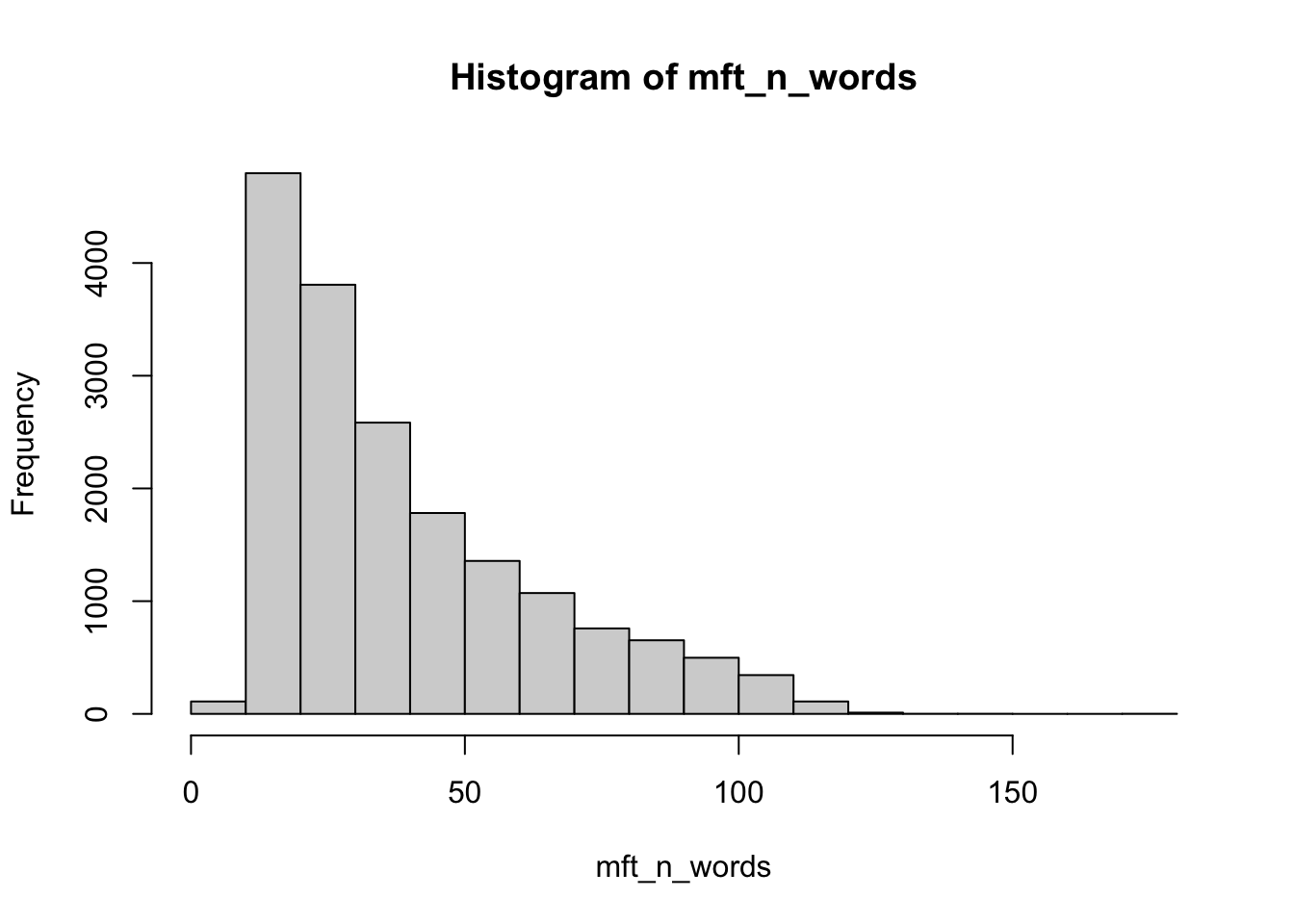
   Min. 1st Qu.  Median    Mean 3rd Qu.    Max. 
   7.00   20.00   31.00   39.09   53.00  177.00

The median length of the comments in the Reddit corpus is 31 words. The figure shows that the distribution of lengths across the corpus is positively skewed, as the mass of the distribution is concentrated on the left.

1.8.1 Create a dictionary

Dictionaries are named lists, consisting of a “key” and a set of entries defining the equivalence class for the given key. In quanteda, dictionaries are created using the dictionary() function. This function takes as input a list, which should contain a number of named character vectors.

For instance, say we wanted to create a simple dictionary for measuring words related to the two courses: quantitative text analysis and causal inference. We would do so by first creating vectors of words that we think measures each concept and store them in a list:

teaching_dictionary_list <- list(qta = c("quantitative", "text", "analysis", "document", "feature", "matrix"),
                                 causal = c("potential", "outcomes", "framework", "counterfactual"))

And then we would pass that vector to the dictionary() function:

teaching_dictionary <- dictionary(teaching_dictionary_list)
teaching_dictionary

Dictionary object with 2 key entries.
- [qta]:
  - quantitative, text, analysis, document, feature, matrix
- [causal]:
  - potential, outcomes, framework, counterfactual

We could then, of course, expand the number of categories and also add other words to each category.

Before starting on the coding questions, take a look at the mft_dictionary.csv file. Do the words associated with each foundation make sense to you? Do any of them not make sense? Remember, constructing a dictionary requires a lot of subjective judgement and the words that are included will, of course, have a large bearing on the results of any analysis that you conduct!

Create a quanteda dictionary object from the words in the mft_dictionary_words data. Your dictionary should have 2 categories – one for the “care” foundation and one for the “sanctity” foundation.

Hint: To do so, you will need to subset the word variable to only those words associated with each foundation.

Reveal code

mft_dictionary_list <- list(
  care = mft_dictionary_words$word[mft_dictionary_words$foundation == "care"],
  sanctity = mft_dictionary_words$word[mft_dictionary_words$foundation == "sanctity"]
  )

mft_dictionary <- dictionary(mft_dictionary_list)
mft_dictionary

Dictionary object with 2 key entries.
- [care]:
  - alleviate, alleviated, alleviates, alleviating, alleviation, altruism, altruist, beneficence, beneficiary, benefit, benefits, benefitted, benefitting, benevolence, benevolent, care, cared, caregiver, cares, caring [ ... and 444 more ]
- [sanctity]:
  - abstinance, abstinence, allah, almighty, angel, apostle, apostles, atone, atoned, atonement, atones, atoning, beatification, beatify, beatifying, bible, bibles, biblical, bless, blessed [ ... and 640 more ]

Use the dictionary that you created in the question above and apply it to the document-feature matrix that you created earlier in this assignment. To do so, you will need to use the dfm_lookup() function. Look at the help file for this function (?dfm_lookup) if you need to.

Reveal code

mft_dfm_dictionary <- dfm_lookup(mft_dfm, mft_dictionary)
mft_dfm_dictionary

Document-feature matrix of: 17,886 documents, 2 features (78.13% sparse) and 8 docvars.
       features
docs    care sanctity
  text1    0        1
  text2    1        0
  text3    1        0
  text4    1        0
  text5    0        1
  text6    0        0
[ reached max_ndoc ... 17,880 more documents ]

The dictionary-dfm that you just created records the count of words in each text that is related to each moral foundations category. As we saw earlier, however, not all texts have the same number of words! Create a new version of the dictionary-dfm which includes the proportion of words in each text that is related to each of the moral foundation categories.

Reveal code

mft_dfm_dictionary_proportions <- mft_dfm_dictionary/mft_n_words

Store the dictionary scores for each foundation as new variables in the original mft_texts data.frame. You will need to use the as.numeric function to coerce each column of the dfm to the right format to be stored in the data.frame.

Reveal code

mft_texts$care_dictionary <- as.numeric(mft_dfm_dictionary_proportions[,1])
mft_texts$sanctity_dictionary <- as.numeric(mft_dfm_dictionary_proportions[,2])

Note that the code here is simply taking the output of applying the dictionaries and assigning those values to the mft_texts data.frame. This just makes later steps of the analysis a little simpler.

1.8.2 Validity checks

Now that we have constructed our dictionary measure, we will conduct some basic validity checks. We will start by directly examining the texts that are scored highly by the dictionaries in each of the categories.

To do so, we need to order the texts by the scores they were assigned by the dictionary analysis. For example, for the “care” foundation, we could use the following code:

mft_texts$text[order(mft_texts$care_dictionary, decreasing = TRUE)][1:5]

the square brackets operator ([]) allows us to subset the mft_texts$text variable
the order() function orders observations according to their value on the mft_texts$care_dictionary variable, and decreasing = TRUE means that the order will be from largest values to smallest values

Find the 5 texts that have the highest dictionary scores for the care and sanctity foundations.

Reveal code

mft_texts$text[order(mft_texts$care_dictionary, decreasing = TRUE)][1:5]

[1] "i doubt she'd want \"help\" from a childhood bully 🙄"                                                                                                        
[2] "We are talking about threats to human safety, not threats to property."                                                                                       
[3] "What guarantees adoptive parents would have been loving? That the child wouldn’t suffer"                                                                      
[4] "The dress design didn’t have anything to do with child sexual assault victims. https://www.papermag.com/alexander-mcqueen-dancing-girls-dress-2645945769.html"
[5] "This right here. Threatening violence of any kind is not ok, sexual rape violence SO not ok."

mft_texts$text[order(mft_texts$sanctity_dictionary, decreasing = TRUE)][1:5]

[1] "hot fucking damn macron this last bit was inspiring as hell"              
[2] "Fuck you. Seriously, fuck you. Get your shit together you fucking junkie."
[3] "Hell yeah! That’s some hardcore nostalgia right there god DAMN."          
[4] "This is so fucking sad. I hate this god damned country"                   
[5] "Holy fuck. This makes OP TA forever. How fucking awful."

Read the texts most strongly associated with both the care and sanctity foundations. Come to a judgement about whether you think the dictionaries are accurately capturing the concepts of care and sanctity.

Reveal code

In many cases these seem like reasonable texts to associate with these categories. Many of the “care” texts do seem to involve descriptions about harm to people, for example. In other cases, the dictionaries seems to be picking up on the wrong thing. For instance, all of the sanctity examples are essentially due to their use of swear words. While swearing might be correlated with moral sensitivity towards sactity issues, it is probably not constitutive of such concerns and so that suggests the sanctity dictionary might be improved.

The mft_texts object includes a series of variables that record the human annotations of which category each text falls into. Use the table() function to create a confusion matrix which compares the human annotations to the scores generated by the dictionary analysis.

Hint: For this comparison, convert your dictionary scores to a logical vector that is equal to TRUE if the text contains any word from a given dictionary, and FALSE otherwise.

Reveal code

care_confusion <- table( 
  dictionary = mft_texts$care_dictionary > 0,
  human_coding = mft_texts$care)
care_confusion

          human_coding
dictionary FALSE  TRUE
     FALSE 11248  2553
     TRUE   1898  2187

sanctity_confusion <- table(
  dictionary = mft_texts$sanctity_dictionary > 0,
  human_coding = mft_texts$sanctity)
sanctity_confusion

          human_coding
dictionary FALSE  TRUE
     FALSE 13268   878
     TRUE   2871   869

For each foundation, what is the accuracy of the classifier? (Look at the lecture notes if you have forgotten how to calculate this!)

Reveal code

# Care
(2187 + 11248)/(2187 + 11248 + 2553 + 1898)

[1] 0.7511461

# Sanctity
(869 + 13268)/(869 + 13268 + 2871 + 878)

[1] 0.7903947

For each foundation, what is the sensitivity of the classifier?

Reveal code

# Care
(2187)/(2187 + 2553)

[1] 0.4613924

# Sanctity
869/(869 + 878)

[1] 0.4974242

For each foundation, what is the specificity of the classifier?

Reveal code

# Care
(11248)/(11248 + 1898)

[1] 0.8556215

# Sanctity
13268/(13268 + 2871)

[1] 0.8221079

What do these figures tell us about the performance of our dictionaries?

Reveal code

Although the accuracy figures are relatively high, the sensitivity scores suggest that the dictionaries are not doing a very good job of picking up on the true “care” and “sanctity” codings in these texts. The dictionaries identify under 50% of the true-positive cases for both concepts.

Note that you can also calculate these statistics very simply by using the caret package.

Reveal code

# install.packages("caret") # Only run this line of code once!
library(caret)

confusionMatrix(care_confusion, positive = "TRUE")

Confusion Matrix and Statistics

          human_coding
dictionary FALSE  TRUE
     FALSE 11248  2553
     TRUE   1898  2187
                                          
               Accuracy : 0.7511          
                 95% CI : (0.7447, 0.7575)
    No Information Rate : 0.735           
    P-Value [Acc > NIR] : 4.343e-07       
                                          
                  Kappa : 0.3317          
                                          
 Mcnemar's Test P-Value : < 2.2e-16       
                                          
            Sensitivity : 0.4614          
            Specificity : 0.8556          
         Pos Pred Value : 0.5354          
         Neg Pred Value : 0.8150          
             Prevalence : 0.2650          
         Detection Rate : 0.1223          
   Detection Prevalence : 0.2284          
      Balanced Accuracy : 0.6585          
                                          
       'Positive' Class : TRUE

confusionMatrix(sanctity_confusion, positive = "TRUE")

Confusion Matrix and Statistics

          human_coding
dictionary FALSE  TRUE
     FALSE 13268   878
     TRUE   2871   869
                                          
               Accuracy : 0.7904          
                 95% CI : (0.7844, 0.7963)
    No Information Rate : 0.9023          
    P-Value [Acc > NIR] : 1               
                                          
                  Kappa : 0.2118          
                                          
 Mcnemar's Test P-Value : <2e-16          
                                          
            Sensitivity : 0.49742         
            Specificity : 0.82211         
         Pos Pred Value : 0.23235         
         Neg Pred Value : 0.93793         
             Prevalence : 0.09767         
         Detection Rate : 0.04859         
   Detection Prevalence : 0.20910         
      Balanced Accuracy : 0.65977         
                                          
       'Positive' Class : TRUE

1.8.3 Applications

With these validations complete (notwithstanding the relatively weak correlation of our dictionary scores with manual codings) we are now in a position to move forward to a simple application.

Calculate the mean care and sanctity dictionary scores for each of the 11 subreddits in the data.

Hint: There are multiple ways of doing this, but one way is to combine the group_by() and summarise() functions described in the Introduction to Tidyverse page of this site.

Reveal code

dictionary_means_by_subreddit <- mft_texts %>%
  group_by(subreddit) %>%
  summarise(care_dictionary = mean(care_dictionary),
            sanctity_dictionary = mean(sanctity_dictionary)) 

dictionary_means_by_subreddit

# A tibble: 11 × 3
   subreddit           care_dictionary sanctity_dictionary
   <chr>                         <dbl>               <dbl>
 1 AmItheAsshole               0.0118              0.00966
 2 Conservative                0.00946             0.0101 
 3 antiwork                    0.0106              0.0120 
 4 confession                  0.0117              0.0127 
 5 europe                      0.00488             0.00453
 6 geopolitics                 0.00394             0.00137
 7 neoliberal                  0.00430             0.00662
 8 nostalgia                   0.00767             0.00959
 9 politics                    0.00923             0.0108 
10 relationship_advice         0.0127              0.0110 
11 worldnews                   0.00651             0.00616

group_by() is a special function which allows us to apply data operations on groups of the named variable (here, we are grouping by subreddit, as we want to know the mean dictionary scores for each subreddit)
summarise() is a function which allows us to calculate various types of summary statistic for our data

Interpret the subreddit averages that you have just constructed.

Reveal code

It is probably easier to display this information in a plot:

dictionary_means_by_subreddit %>%
  # Transform the data to "long" format for plotting
  pivot_longer(-subreddit) %>%
  # Use ggplot
  ggplot(aes(x = name, y = subreddit, fill = value)) + 
  # geom_tile creates a heatmap
  geom_tile() + 
  # change the colours to make them prettier
  scale_fill_gradient(low = "white", high = "purple") + 
  # remove the axis labels
  xlab("") + 
  ylab("")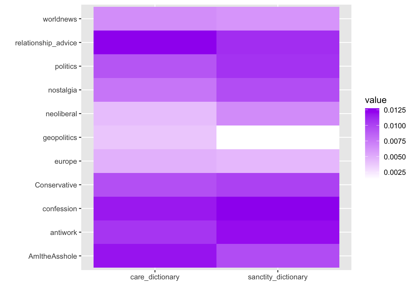

The “geopolitics” subbreddit appears to feature very little language related to sanctity; the “confession” subreddit uses lots of language related to sanctity

Care-based language is prevalent in the “relationship_advice” and “AmItheAsshole” subreddits

What is the correation between the dictionary scores for care and sanctity? Are the foundations strongly related to each other?

Hint: The correlation between two variables can be calculated using the cor() function.

Reveal code

cor(mft_texts$care_dictionary,mft_texts$sanctity_dictionary)

[1] 0.03435137

No, the correlation between care- and sanctity-based language is very low.

1.9 Homework

Replicate the analyses in this assignment for the other three foundations (fairness, loyalty, and authority) included. Create a plot showing the average dictionary score for each foundation, for each subreddit.

Reveal code

mft_dictionary_list <- list(
  care = mft_dictionary_words$word[mft_dictionary_words$foundation == "care"],
  sanctity = mft_dictionary_words$word[mft_dictionary_words$foundation == "sanctity"],
  authority = mft_dictionary_words$word[mft_dictionary_words$foundation == "authority"],
  fairness = mft_dictionary_words$word[mft_dictionary_words$foundation == "fairness"],
  loyalty = mft_dictionary_words$word[mft_dictionary_words$foundation == "loyalty"]
  )

mft_dictionary <- dictionary(mft_dictionary_list)

mft_dfm_dictionary <- dfm_lookup(mft_dfm, mft_dictionary)

mft_dfm_dictionary_proportions <- mft_dfm_dictionary/mft_n_words

mft_texts$care_dictionary <- as.numeric(mft_dfm_dictionary_proportions[,1])
mft_texts$sanctity_dictionary <- as.numeric(mft_dfm_dictionary_proportions[,2])
mft_texts$authority_dictionary <- as.numeric(mft_dfm_dictionary_proportions[,3])
mft_texts$fairness_dictionary <- as.numeric(mft_dfm_dictionary_proportions[,4])
mft_texts$loyalty_dictionary <- as.numeric(mft_dfm_dictionary_proportions[,5])

dictionary_means_by_subreddit <- mft_texts %>%
  group_by(subreddit) %>%
  summarise(care_dictionary = mean(care_dictionary),
            sanctity_dictionary = mean(sanctity_dictionary),
            authority_dictionary = mean(authority_dictionary),
            fairness_dictionary = mean(fairness_dictionary),
            loyalty_dictionary = mean(loyalty_dictionary)) 


dictionary_means_by_subreddit %>%
  # Transform the data to "long" format for plotting
  pivot_longer(-subreddit) %>%
  # Use ggplot
  ggplot(aes(x = name, y = subreddit, fill = value)) + 
  # geom_tile creates a heatmap
  geom_tile() + 
  # change the colours to make them prettier
  scale_fill_gradient(low = "white", high = "purple") + 
  # remove the axis labels
  xlab("") + 
  ylab("")

Write a short new dictionary that captures a concept of interest to you. Implement this dictionary using quanteda and apply it to the Moral Foundations Reddit Corpus. Create one plot communicating something interesting that you have found from this exercise.

Upload both of your plots to this Moodle page.

Reveal code

You could have specified any dictionary here. Some of the more creative ones this week included a dictionary related to relief and stress; a dictionary related to Maslow’s theory of need; and dictionaries that captured words related to feminist issues. Good work all!

1.1 Lecture slides

1.2 Introduction

1.3 Measuring Moral Sentiment

1.3.1 Data

1.3.2 Packages

1.4 Creating a corpus

1.4.1 Getting Help

1.4.2 Making a corpus and corpus structure

1.5 Tokenizing texts

1.6 Creating a dfm()

1.7 Pipes

1.8 Descriptive Statistics

1.8.1 Create a dictionary

1.8.2 Validity checks

1.8.3 Applications

1.9 Homework

1.6 Creating a `dfm()`