2 Causality I

2.1 Seminar

In the seminar this week, we will cover the following topics:

Thinking about how we can use experimental data to make causal claims
Folders, files and working directories
Loading data using read.csv()
Missing data

Before coming to the seminar

Please read chapter 3, in Thinking Clearly with Data. (essential)
Please read chapter 2, “Causality”, in Quantitative Social Science: An Introduction. (recommended)

Files and folders

It is sensible when you start any data analysis project to make sure your computer is set up in an efficient way. Last week, you should have created a script with the name seminar1.R. Hopefully, you will have saved this somewhere sensible! Our suggestion is that you create a folder on your computer with the name PUBL0055 which you can save all your scripts in throughout the course. If you didn’t set up a folder like that on your computer, do so now.

Once you have a folder with the name PUBL0055, make sure your seminar1.R file is saved within it. Now create a new R script, and save that in your folder with the name seminar2.R. Use this script to record all the code that you are working on this week. Each week you should start a new script and save it in this folder.

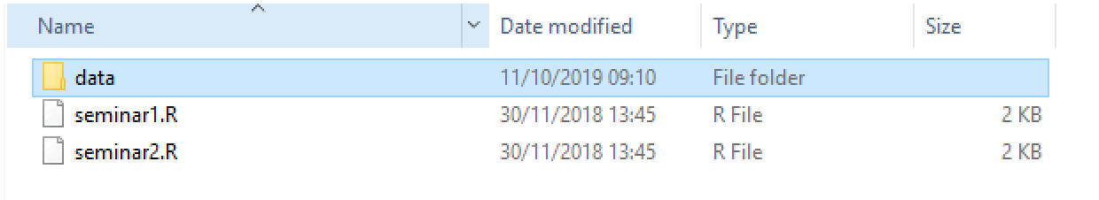
This week we will also be loading some data into R for analysis. Let’s add a subfolder into your main PUBL0055 folder, and give it the name data. The contents of your folder should now look something like this if you are working on a Mac:

And like this if you are working on a PC:

Working directories

If you open Rstudio, the first thing you should include at the beginning of your script is code to set the “working directory”. This tells R where to look for scripts and data when you run your code. If you are working on a Mac and have saved your PUBL0055 folder on the desktop of your computer, for example, then you can tell R to work from that folder by running the following code:

# set working directory
setwd("~/Desktop/PUBL0055")

# (If you're having problems, you can run getwd() to identify where on your 
# computer R thinks it's working)

If you were working on a Windows PC, you might use:

setwd("C:/Desktop/PUBL0055")

You can adjust the code above to direct R to look to wherever the relevant folwder is stored on your computer. For instance, if your PUBL0055 folder is kept inside your UCL folder, you could use setwd("~/Desktop/UCL/PUBL0055"), and so on.

Loading data

Save transphobia.csv into the data folder that you created earlier in the seminar. Then load the R script that you are using for this week. Now load the data using the read.csv() function:

transphobia <- read.csv("data/transphobia.csv")

This function loads the data stored in "transphobia.csv" into R, and then we are using the assignment operator – <- – that we learned last week to create a new object. Once the data is loaded, you should see the transphobia object appear in the Environment pane of Rstudio.

As you can see from the output above, this data has 488 rows (units), and 11 columns (variables). We will describe these below.

2.1.1 Contact and Transphobia

Can transphobia be reduced through in-person conversations and perspective-taking exercises, or active processing? Following up on previous research that had been shown to be fabricated, two researchers conducted a door-to-door canvassing experiment in South Florida targeting anti-transgender prejudice in order to answer this question. Canvassers held single, approximately 10-minute conversations that encouraged actively taking the perspective of others with voters to see if these conversations could markedly reduce prejudice.

Broockman, David and Joshua Kalla. 2016. “Durably reducing transphobia: a field experiment on door-to-door canvassing.” Science, Vol. 352, No. 6282, pp. 220-224.

In the experiment, the authors first recruited registered voters ($n=68378$) via mail for an online baseline survey, presented as the first in a series of surveys. They then randomly assigned respondents of this baseline survey ($n=1825$) to either a treatment group targeted with the intervention ($n=913$) or a placebo group targeted with a conversation about recycling ($n=912$). For the intervention, 56 canvassers first knocked on voters’ doors unannounced. Then, canvassers asked to speak with the subject on their list and confirmed the person’s identity if the person came to the door. A total of several hundred individuals ($n=501$) came to their doors in the two conditions. For logistical reasons unrelated to the original study, we further reduce this dataset to ($n=488$) which is the full sample that appears in the transphobia.csv data.

The canvassers then engaged in a series of strategies previously shown to facilitate active processing under the treatment condition: canvassers informed voters that they might face a decision about the issue (whether to vote to repeal the law protecting transgender people); canvassers asked voters to explain their views; and canvassers showed a video that presented arguments on both sides. Canvassers defined the term “transgender” at this point and, if they were transgender themselves, noted this. The canvassers next attempted to encourage “analogic perspective-taking”. Canvassers first asked each voter to talk about a time when they themselves were judged negatively for being different. The canvassers then encouraged voters to see how their own experience offered a window into transgender people’s experiences, hoping to facilitate voters’ ability to take transgender people’s perspectives. The intervention ended with another attempt to encourage active processing by asking voters to describe if and how the exercise changed their mind. All of the former steps constitutes the “treatment.”

The placebo group was reminded that recycling was most effective when everyone participates. The canvassers talked about how they were working on ways to decrease environmental waste and asked the voters who came to the door about their support for a new law that would require supermarkets to charge for bags instead of giving them away for free. This was meant to mimic the effect of canvassers interacting with the voters in face-to-face conversation on a topic different from transphobia.

The authors then asked the individuals who came to their doors in either condition ($n=488$) to complete follow-up online surveys via email presented as a continuation of the baseline survey. These follow-up surveys began 3 days, 3 weeks, 6 weeks, and 3 months after the intervention when the baseline survey was also conducted. For the purposes of this exercise, we will be using the tolerance.t# variables (where # is 0 through 4) as the main outcome variables of interest. The authors constructed these dependent variables tolerance.t# as indexes by using several other measures that are not included in this exercise. In building this index, the authors scaled the variables such that they have a mean of 0 and standard deviation of 1 for the placebo group. Higher values indicate higher tolerance, lower values indicate lower tolerance relative to the placebo group.

The data set is the file transphobia.csv. Variables that begin with vf_ come from the voter file. Variables in this dataset are described below:

Name	Description
`vf_age`	Age
`vf_party`	Party: `D`=Democrats, `R`=Republicans and `N`=Independents
`vf_racename`	Race: `African American`, `Caucasian`, `Hispanic`
`vf_female`	Gender: `1` if female, `0` if male
`treat_ind`	Treatment assignment: `1`=treatment, `0`=placebo
`treatment.delivered`	Intervention was actually delivered (=`TRUE`) vs. was not (=`FALSE`)
`tolerance.t0`	Outcome tolerance variable at Baseline
`tolerance.t1`	(see above) Captured at 3 days after Baseline
`tolerance.t2`	(see above) Captured at 3 weeks after Baseline
`tolerance.t3`	(see above) Captured at 6 weeks after Baseline
`tolerance.t4`	(see above) Captured at 3 months after Baseline

To get a sense of what this data.frame contains, use the functions below:

head(transphobia) – shows the first six (by default) rows of the data
str(transphobia) – shows the “structure” of the data
View(transphobia) – opens a spreadsheet-style viewer of the data

Question 1

For this question, we will learn to use the table() function, which provides counts of the number of observations in our data that take distinct values for a given variable or pair of variables.

The table function can be used to provide the number of respondents that fall into a given category for a single variable. To do this, simply provide the name of the variable of interest as the first argument to the table function:

table(data_name$variable_name)

Or it can be used to provide the number of respondents that fall into the combination of categories of two different variables. To do this, provide both variable names to the table function:

table(data_name$variable_name_one, data_name$variable_name_two)

Look at the help file for this function for more information (?help).

Use this function to answer the following questions:

How many respondents were chosen to have a canvasser come to their door to talk to them about transphobia? How many were targeted with a conversation about recycling (the placebo group)?
How many respondents were Democrats? How many were not?
Of the respondents that were assigned the treatment (i.e., the transphobia intervention), how many were Democrats?
Of the respondents that were in the placebo group, how many were Democrats?

Reveal answer

table(transphobia$treat_ind)

## 
##   0   1 
## 252 236

Using the table function shows that 252 respondents were selected to receive the placebo intervention (the recycling conversation) and 236 respondents were selected to receive the treatment (the transphobia conversation).

table(transphobia$vf_party)

## 
##   D   N   R 
## 242 120 126

242 respondents were Democrats, 126 were Republicans.

3 and 4

table(transphobia$treat_ind, transphobia$vf_party)

##    
##       D   N   R
##   0 117  64  71
##   1 125  56  55

When applied to two variables, the counts for the first variable are indicated by the rows of the resulting matrix, and the counts for the second variable are indicated by the columns. So, in this case, of the 236 respondents that received the treatment (second row), 125 were Democrats and 55 were Republicans. By contrast, 117 of the respondents that were targeted with the recycling conversation were Democrats and 71 were Republicans.

Question 2

When attempting to answer the research question about whether transphobia can be reduced through in-person conversations, is confounding something you should be worried about?

Reveal answer

Absolutely! For example, I should be worried that people who are more likely to have conversations with transgender people tend to be more tolerant even before the conversation. If that is the case, just comparing people who have more conversations with transgender people to people who have fewer conversations with transgender people would give me a biased estimate of the average treatment effect.

Question 3

In this question, we will investigate whether respondents who were selected to receive the intervention (a conversation about transphobia) were more likely to be female than respondents selected to receive the recycling conversation.

Conduct comparisons between treated and untreated observations in terms of the mean level of female. What do you find?

Reveal answer

mean(transphobia$vf_female[transphobia$treat_ind == 1])
mean(transphobia$vf_female[transphobia$treat_ind == 0])

## [1] 0.5508475
## [1] 0.5952381

55% of treated respondents were female, and 60% of respondents who received the recycling conversation were female. This suggests (as we would expect in a randomized experiment), that the share of female respondents among treated individuals is similar to the share of female respondents among the untreated individuals.

Question 4

Compare the average (mean) tolerance for treated and untreated respondents 3 days after the intervention using the tolerance.t1 and the treat_ind variables. Note that for this question, you will have to use the mean function to calculate the mean of various subsets of the data. However, you will find that if you simply apply the mean function to the transphobia$tolerance.t1 variable it does not produce the desired result:

mean(transphobia$tolerance.t1)

## [1] NA

R returns NA because for some respondents (those that did not participate in the survey 3 days after the intervention) we have no information on the level of tolerance. In short, NA is the R value for missing data. We can tell the mean() function to estimate the mean only for those respondents that we do have data for, and ignore the other respondents by setting an additional argument for the mean function: mean(dataset_name$var_name, na.rm = TRUE).

mean(transphobia$tolerance.t1, na.rm = TRUE)

## [1] 0.07688603

Based on your comparison, would you conclude that the transphobia conversation had an impact on tolerance? Why or why not?

Hint: You can use the same coding structure that you used in your answers to question 1 and 2 to help here.

Reveal answer

tolerance_treated <- mean(transphobia$tolerance.t1[transphobia$treat_ind == 1], na.rm=TRUE)
tolerance_recycling <- mean(transphobia$tolerance.t1[transphobia$treat_ind == 0], na.rm=TRUE)

tolerance_treated  - tolerance_recycling

## [1] 0.1443226

The estimated difference in means reveals that respondents who were selected to receive the transphobia conversation on average exhibit slightly higher levels of tolerance than respondents who were assigned a recycling conversation. The average level of tolerance after the intervention among treated respondents is 0.15. The average level of tolerance 3 days after the intervention among respondents who did not receive the treatment was 0.01. By itself, this comparison suggests that conversations with canvassers about transphobia may increase tolerance toward transgender people, although the effect is not large.

Question 5

In the question above, we used the variable treat_ind to calculate the difference in means for the level of tolerance three days after the conversation, depending on whether an individual received a conversation about transphobia or recycling. Is this difference in means likely to represent the causal effect of a conversation about transphobia? Why or why not? Which assumptions are required to give this difference a causal interpretation? Give some thought to these questions, and discuss your reasoning with the people next to you.

Reveal answer

Recall the discussion of confounding from the lecture. There we argued that making causal statements on the basis of evidence drawn from observational studies is difficult because confounding differences between treatment and control observations mean that the difference in means can result in a biased estimate of the average treatment effect. In essence, to make a causal statement on the basis of observational evidence, one needs to assume that there are no confounding differences between treatment and control groups. However, if an experiment is conducted in which individuals are randomly chosen to receive the treatment or not (i.e., they are assigned to a treatment or a control group), the groups should be similar, on average, in terms of all characteristics (both observed and unobserved). Accordingly, the only way in which these groups differ on average is with respect to whether or not they received the treatment or not.

In this case, we have a randomised experiment. Put another way, if respondents were randomly assigned into treatment and control groups, it should not be the case that respondents allocated to the treatment group had higher levels of tolerance before the intervention.

Question 6

Create a new variable called participated.t1 by including information about whether or not the respondent participated in the first follow up survey (3 days after the intervention) using the following code:

# is.na() tells us where there is a missing value in the variable 
# tolerance.t1 (we are missing values where the respondent did not 
# participate in the survey at this time)
transphobia$participated.t1 <- !is.na(transphobia$tolerance.t1)

Here we are using the assignment operator to create a new variable in our transphobia data. If this new variable equals TRUE, this indicates that this individual participated in the survey (the value in tolerance.t1 is NOT (!) NA). If the value in the new variable equals FALSE, this indicates that the individual did not participate in the follow up survey (the value in the tolerance.t1 variable is NA)

Did the intervention have an effect of whether or not a respondent participated in the survey 3 days after the intervention?

Hint: You can use the same coding structure that you used in your answers to question 4 to help here.

Reveal answer

transphobia$participated.t1 <- !is.na(transphobia$tolerance.t1)

participation_treated <- mean(transphobia$participated.t1[transphobia$treat_ind == 1], na.rm=TRUE)
participation_recycling <- mean(transphobia$participated.t1[transphobia$treat_ind == 0], na.rm=TRUE)

participation_treated  - participation_recycling

## [1] -0.05044391

The estimated difference in means reveals that respondents who were selected to receive the transphobia conversation are slightly less likely to participate in the survey 3 days later. The average share of participants among treated individuals is 83.05 and the share of participants among untreated individuals is 88.1. By itself, this comparison suggests that conversations with canvassers about transphobia may have affected respondents’ likelihood to participate in the follow up survey.

2.2 Homework

2.2.1 Demographic Change and Exclusionary Attitudes

This week’s homework uses data based on: Enos, R. D. 2014. “Causal Effect of Intergroup Contact on Exclusionary Attitudes.” Proceedings of the National Academy of Sciences 111(10): 3699–3704. You can download this data from the link at the top of the page. Once you have done so, store it in the data subfolder you created earlier. Then start a new R script which you should save as homework2.R.

Enos conducted a randomized field experiment assessing the extent to which individuals living in suburban communities around Boston, Massachusetts, were affected by exposure to demographic change.

Subjects in the experiment were individuals riding on the commuter train line and were overwhelmingly white. Every morning, multiple trains pass through various stations in suburban communities that were used for this study. For pairs of trains leaving the same station at roughly the same time, one was randomly assigned to receive the treatment and one was designated as a control. By doing so all the benefits of randomization apply for this dataset.

The treatment in this experiment was the presence of two native Spanish-speaking ‘confederates’ (a term used in experiments to indicate that these individuals worked for the researcher, unbeknownst to the subjects) on the platform each morning prior to the train’s arrival. The presence of these confederates, who would appear as Hispanic foreigners to the subjects, was intended to simulate the kind of demographic change anticipated for the United States in coming years. For those individuals in the control group, no such confederates were present on the platform. The treatment was administered for 10 days. Participants were asked questions related to immigration policy both before the experiment started and after the experiment had ended. The names and descriptions of variables in the data set boston.csv are:

Name	Description
`age`	Age of individual at time of experiment
`male`	Sex of individual, male (1) or female (0)
`income`	Income group in dollars (not exact income)
`white`	Indicator variable for whether individual identifies as white (1) or not (0)
`college`	Indicator variable for whether individual attended college (1) or not (0)
`usborn`	Indicator variable for whether individual is born in the US (1) or not (0)
`treatment`	Indicator variable for whether an individual was treated (1) or not (0)
`ideology`	Self-placement on ideology spectrum from Very Liberal (1) through Moderate (3) to Very Conservative (5)
`numberim.pre`	Policy opinion on question about increasing the number immigrants allowed in the country from Increased (1) to Decreased (5)
`numberim.post`	Same question as above, asked later
`remain.pre`	Policy opinion on question about allowing the children of undocumented immigrants to remain in the country from Allow (1) to Not Allow (5)
`remain.post`	Same question as above, asked later
`english.pre`	Policy opinion on question about passing a law establishing English as the official language from Not Favor (1) to Favor (5)
`english.post`	Same question as above, asked later

Question 1

The benefit of randomly assigning individuals to the treatment or control groups is that the two groups should be similar, on average, in terms of their other characteristics, or “covariates”. This is referred to as “covariate balance.”

Use the mean function to determine whether the treatment and control groups are balanced with respect to the age (age) and income (income) variables. Also, compare the proportion of males (male) in the treatment and control groups. Interpret these numbers.

(Hint: to calculate the proportion of observations with a given attribute on a binary variable, you can just use mean(data_frame_name$variable_name).)

Reveal answer

## Load data

boston <- read.csv("data/boston.csv", head = TRUE)

## Mean age for treatment and control units

mean_age_treated <- mean(boston$age[boston$treatment == 1])
mean_age_control <- mean(boston$age[boston$treatment == 0])

mean_age_treated - mean_age_control

## [1] -3.912299

## Mean income levels for treatment and control units

mean_income_treated <- mean(boston$income[boston$treatment == 1])
mean_income_control <- mean(boston$income[boston$treatment == 0])

mean_income_treated - mean_income_control

## [1] -15972.59

## Proportion "male" for treatment and control units

prop_male_treated <- mean(boston$male[boston$treatment == 1])
prop_male_control <- mean(boston$male[boston$treatment == 0])

prop_male_treated - prop_male_control

## [1] -0.06096257

Despite the randomization of treatment assignment, there are some differences in the average characteristics of treatment and control units. For example, the average age of treated individuals is 40.4, where is is 44.3 for control units. Similarly, while 53% of treated individuals are male, 59% of control individuals are male. Most notably, the average income of the treated group is approximately $16000 lower than it is for the control group.

Overall, while the treatment and control groups are relatively well balanced, there remain some potentially problematic confounding differences between these groups. This is an example of the point made in lecture: although randomized experiments provide unbiased estimates on average, any given instance of randomization may not create perfect balance across all covariates. That is, you might be unlucky! That is why it is often important to run replication studies of randomized experiments to ensure that the results we obtain are not simply because we were lucky/unlucky in any particular randomization of the treatment.

Question 2

Individuals in the experiment were asked “Do you think the number of immigrants from Mexico who are permitted to come to the United States to live should be increased, left the same, or decreased?” The response to this after the experiment is in the variable numberim.post. The variable is coded on a 1 – 5 scale. Responses with values of 1 are inclusionary (‘pro-immigration’) and responses with values of 5 are exclusionary (‘anti-immigration’). Calculate the mean value of this variable for the treatment and control groups. What is the difference in means? What does the result suggest about the effects of intergroup contact on exclusionary attitudes?

Reveal answer

## Calculate the mean in each group (note that na.rm = T is required here)

treat_mean <- mean(boston$numberim.post[boston$treatment == 1], na.rm = T)
control_mean <- mean(boston$numberim.post[boston$treatment == 0], na.rm = T)

## Calculate the difference in means

treat_mean - control_mean

The difference in means suggests that the treatment group reported, on average, 0.39 points higher on the 5 point scale than the control group. As higher values of the outcome variable suggest more exclusionary attitudes, this suggests that contact with the Spanish speaking confederates increases exclusionary attitudes, at least in this experiment. Because the responses of individuals in the treatment group were more exclusionary than the control group, we would conclude on the basis of this experiment that exposure to potential demographic changes cause increases in exclusionary attitudes.

Question 3

Does having attended college influence the effect of being exposed to ‘outsiders’ on exclusionary attitudes? Another way to ask the same question is this: is there evidence of a differential impact of treatment, conditional on attending college versus not attending college? Calculate the difference in means between treatment and control observations amongst those who attended college and those who did not. Interpret your results.

(Hint: You may want to subset the data using more than one logical condition here. For example, if I wanted to subset the data to include only the observations which were treated and went to college, I could use boston$numberim.post[boston$treatment == 1 & boston$college == 1].)

Reveal answer

## First calculate the mean outcome for treatment and control observations *who went to college*

treat_college_mean <- mean(boston$numberim.post[boston$treatment == 1 & boston$college == 1],
                     na.rm = TRUE)

control_college_mean <- mean(boston$numberim.post[boston$treatment == 0 & boston$college == 1],
                     na.rm = TRUE)

## Now calculate the mean outcome for treatment and control observations *who did not go to college*

treat_nocollege_mean <- mean(boston$numberim.post[boston$treatment == 1 & boston$college == 0],
                     na.rm = TRUE)

control_nocollege_mean <- mean(boston$numberim.post[boston$treatment == 0 & boston$college == 0],
                     na.rm = TRUE)


## Difference in means for college observations

diff_college <- treat_college_mean - control_college_mean
diff_college

## Difference in means for non-college observations

diff_nocollege <- treat_nocollege_mean - control_nocollege_mean
diff_nocollege

## [1] 0.4929467
## [1] -0.4285714

The average treatment effect (using the numberim.post variable) among those with a college education is an increase in exclusionary attitudes of about 0.49 points. Among those without a college education, there is a decrease in exclusionary attitudes of about .43 points. Both of these effects are on a 5 point scale. At face value this suggests that the effects of “outgroup” contact on exclusionary attitudes might differ according to education.

Question 4

Calculate the number of observations used to calculate each of the mean outcome values you used in the answer for question 3. What does this suggest about the reliability of the conclusions you drew from that analysis?

Reveal answer

table(boston$treatment, boston$college)

##    
##      0  1
##   0  7 61
##   1  8 47

Using the table function reveals that some of the averages calculated above are based on a very small number of observations. In particular, the vast majority of the data in our sample is of individuals who have college degrees. Only 15 individuals are not college educated. Accordingly, we might worry that the averages we have calculated above for non-college individuals may capture idiosyncrasies of these individuals rather than anything general about the broader population of non-college educated individuals.

How many observations is “enough”? The short answer is: it depends. The long answer: we will cover this extensively in future weeks!