8 Uncertainty I (Sampling)
8.1 Overview
In the lecture this week, we changed focus from thinking about causal inference, and started instead to think about statistical inference. In particular, we considered the problem of making inferences about population-level quantities of interest when all we can observe is a sample of data that is taken from that population. We discussed sampling variation, and the concept of the sampling distribution: the distribution of estimates that would result from repeatedly sampling from the population and calculating our quantity of interest for every sample. We saw that while we cannot observe the sampling distribution directly, we know that it will always be approximately normally distributed (thanks to the central limit theorem), and that we can estimate the standard deviation of the sampling distribution by calculating the standard error. Finally, we saw that we can quantify the uncertainty in our estimates by constructing a confidence interval.
In the seminar this week, we will:
- Practice calculating the difference in means, the standard error, and various confidence intervals.
- Practice interpreting those quantities.
- Learn to use the
t.test()function to calculate confidence intervals. - Learn more about R’s plotting functions.
Before coming to the seminar, please read:
Chapter 6, sections “Introduction” until “Quantifying Precision”, in Bueno de Mesquita & Fowler (2021) Thinking Clearly with Data (essential)
Section 6.3.4, 6.4.2, and 7.1, in Quantitative Social Science: An Introduction (recommended)
8.2 Seminar
In this exercise, we examine the hypothesis that family members of people who died in the terrorist attacks of 9/11 subsequently became more politically engaged. Estimating the specific and long-term political effects of terrorist attacks on the families of victims is important for understanding the effects of terrorist activities. This exercise is based on: Hersh, E. D. 2013. “Long-Term Effect of September 11 on the Political Behavior of Victims’ Families and Neighbors.” Proceedings of the National Academy of Sciences 110(52): 20959–63.
Download the data file, victims.csv, from the link above, and store it in your data folder as you have done in previous weeks. Then load the data into R:
The data contains observations of 7054 individuals and includes the following variables:
| Name | Description |
|---|---|
treatment |
Families of victims (1) vs control group (0) |
ge2000 |
Voting in the 2000 general election (1=voted, 0 = did not vote) |
ge2002 |
Voting in the 2002 general election (1=voted, 0 = did not vote) |
ge2004 |
Voting in the 2004 general election (1=voted, 0 = did not vote) |
ge2006 |
Voting in the 2006 general election (1=voted, 0 = did not vote) |
ge2008 |
Voting in the 2008 general election (1=voted, 0 = did not vote) |
ge2010 |
Voting in the 2010 general election (1=voted, 0 = did not vote) |
ge2012 |
Voting in the 2012 general election (1=voted, 0 = did not vote) |
fam.members |
Number of family members living with voter at their address |
age |
Voter’s age |
pct.white |
Proportion of non-Hispanic white voters living on the same block |
median.income |
Median income of voters living on the same block |
female |
1 if the voter is female, 0 otherwise |
The treatment group in this study (i.e. observations where treatment = 1) are individuals living in New York who were related to people who died in the 9/11 attacks. The control group (treatment = 0) is also made up of individuals living in New York who were similar to the treated group with regard to demographics, prior political activities, and family and neighbourhood characteristics, but who did not have family members die in the attacks.
For the purposes of this exercise, we will treat the data as being a random sample which is drawn from a broader population of units.
Question 1
Use the difference in means to estimate “the average treatment effect” of being a family member of a victim on voter turnout in 2000 (i.e. the year before the 9/11 attacks). Is it always the case that the difference in means that you calculate in this sample will be equal to the difference in means in the population? Why or why not?
Bonus question: Discuss with your neighbour what needs to be true in order for us to be able to estimate the causal effect of being a family member of a victim, and whether this assumption is likely to hold in this data.
Reveal answer
# Average turnout treatment group
treat_mean_00 <- mean(victims$ge2000[victims$treatment == 1])

# Average turnout control group
control_mean_00 <- mean(victims$ge2000[victims$treatment == 0])

# Difference in means
diff_00 <- treat_mean_00 - control_mean_00
diff_00
## [1] -0.001831524The difference in means here suggests that turnout was 0.18 percentage points lower for the treated group than the control group.
No, sampling variation means that the difference in means that we calculate in any particular sample will be different from the difference in means that exists in the population. Sometimes we will overestimate the difference in means (it will be too big), and sometimes we will underestimate the difference in means (it will be too small). That is the case even if we treat this sample as a random sample of the population.
Bonus question In the description of our data that we stated that “The control group (treatment = 0) is also made up of individuals living in New York who were similar to the treated group with regard to demographics, prior political activities, and family and neighbourhood characteristics, but who did not have family members die in the attacks.” In other words, this means that the treatment and control groups are similar in all relevant observable and unobservable characteristics (i.e., not systematically different from each other) except the treatment. If this is indeed the case, we can conclude that the unconfoundedness assumption is met. In our data, we should see that the treatment and control groups are balanced in pre-treatment characteristics, including their pre-treatment voting behaviour.
Question 2
- Calculate the standard error of the difference in means. Remember, the formula for the standard error of the difference in means is: \[ SE(\hat{Y}_{X=1} - \hat{Y}_{X=0}) = \sqrt{\frac{Var(Y_{X=1})}{n_{X=1}} + \frac{Var(Y_{X=0})}{n_{X=0}}} \]
Reveal answer
# Calculate the variance for the treatment group
treat_var_00 <- var(victims$ge2000[victims$treatment == 1])

# Calculate the variance for the control group
control_var_00 <- var(victims$ge2000[victims$treatment == 0])

# Calculate the sum of observations in the treatment group
treat_n_00 <- sum(victims$treatment == 1)

# Calculate the sum of observations in the control group
control_n_00 <- sum(victims$treatment == 0)

# Calculate the standard error of the difference in means
st_err_00 <- sqrt(treat_var_00/treat_n_00 + control_var_00/control_n_00)
st_err_00
## [1] 0.01550951- Calculate the 95% confidence interval, using the appropriate critical values from the standard normal distribution. Remember, the formula for the 95% confidence interval is: \[ \bar{Y}_{X = 1} - \bar{Y}_{X = 0} \pm 1.96 * SE(\bar{Y}_{X = 1} - \bar{Y}_{X = 0}) \]
Reveal answer
# Calculate the upper confidence interval
upper_00_95 <- diff_00 + 1.96 * st_err_00
upper_00_95

# Calculate the lower confidence interval
lower_00_95 <- diff_00 - 1.96 * st_err_00
lower_00_95
## [1] 0.02856712
## [1] -0.03223017- Considering the difference in means from question 1 and the confidence interval you just computed, what can we conclude about the difference in turnout between the treatment and control groups before 9/11?
Reveal answer
The difference in means for the year 2000, before the 9/11 attacks took place functions as a “placebo” test in this example. That is, there is no reason to think that the family members of 9/11 victims should differ in their political behaviour in elections before 9/11 from individuals who did not know someone who died in the attacks. In other words, if the treatment and control groups were similar prior to the administration of treatment, then the treatment effect for 2000 should be equal to zero. Although the difference in means calculation shows a very small difference between treatment and control groups in 2000 – -0.002 – (i.e. the difference in means is not exactly zero in this sample), the 95% confidence interval ranges from -0.032 to 0.029.
This means that if we were to randomly sample from our population many, many times and always calculated the difference in means and the corresponding 95% confidence interval, the 95% confidence interval would include the population difference in turnout 95% of times. As this interval includes the value of zero, we conclude that there is no statistically significant difference between treatment and control turnout rates in the election in 2000.
Question 3
Repeat the steps above, again comparing treatment and control observations and calculating the 95% confidence interval, but in this case for turnout the 2002 election. What is the substantive conclusion that you draw from this analysis?
Reveal answer
# Difference in means
treat_mean_02 <- mean(victims$ge2002[victims$treatment == 1])
control_mean_02 <- mean(victims$ge2002[victims$treatment == 0])
diff_02 <- treat_mean_02 - control_mean_02
diff_02

# Standard error
treat_var_02 <- var(victims$ge2002[victims$treatment == 1])
control_var_02 <- var(victims$ge2002[victims$treatment == 0])

treat_n_02 <- sum(victims$treatment == 1)
control_n_02 <- sum(victims$treatment == 0)

st_err_02 <- sqrt(treat_var_02/treat_n_02 + control_var_02/control_n_02)
st_err_02

# 95% confidence interval
upper_02_95 <- diff_02 + 1.96 * st_err_02
upper_02_95
lower_02_95 <- diff_02 - 1.96 * st_err_02
lower_02_95
## [1] 0.01902632
## [1] 0.01540058
## [1] 0.04921145
## [1] -0.01115881Consistent with the hypothesis, we find a positive difference in means for the 2002 election. On average, the turnout rate of individuals in the control group was 37.74%, whereas the turnout rate of individuals who were related to people who had died in the 9/11 attacks was 39.64%, implying a small positive sample average treatment effect.
However, the confidence interval that we have calculated ranges from -0.01 to 0.05 and therefore contains zero. This implies that we cannot be confident that the true treatment effect in the population is positive.
Question 4
- Calculate the difference in mean turnout (and the associated 95% confidence intervals) between treatment and control units for all other election years in the data (2004, 2006, 2008, 2010, and 2012).
Rather than calculating the confidence intervals “by hand” as you did above, here use the t.test() function. The main arguments for this function are given in the table below:
| Arguments | Description |
|---|---|
x |
The outcome values for one group of observations. |
y |
The outcome values for another group of observations. |
conf.level |
The level of confidence that we want to use to construct the confidence intervals. |
Note that you can extract the estimated confidence intervals from the output of t.test() by using the $ sign. For instance, if your save the output of the function as t_test_output, then you can extract the confidence intervals by using t_test_output$conf.int.
Reveal answer
First, let’s confirm that the
t.test()function provides the same results for the confidence intervals as those we calculated above:
# T-test for average turnout in treatment and control for 2000 election
t_test_00 <- t.test(x = victims$ge2000[victims$treatment == 1],
                    y = victims$ge2000[victims$treatment == 0],
                    conf.level = 0.95)

# Extract confidence intervals & compare to manual calculations
t_test_00$conf.int

lower_00_95
upper_00_95
## [1] -0.03225057 0.02858752
## attr(,"conf.level")
## [1] 0.95
## [1] -0.03223017
## [1] 0.02856712Yes, the confidence intervals are the same up to the 4th decimal place. The small differences in the values after that point come from the fact that the
t.test()function assumes that the sampling distribution for the difference in means follows a “t-distribution”, whereas we assumed that the sampling distribution follows a normal distribution. When the sample size is large, as it is here, these two approaches will always result in very similar values.
Now let’s calculate the confidence intervals for all the other years in the sample:
# 2002 election
t_test_02 <- t.test(x = victims$ge2002[victims$treatment == 1],
                    y = victims$ge2002[victims$treatment == 0],
                    conf.level = 0.95)

t_test_02$conf.int

# 2004 election
t_test_04 <- t.test(x = victims$ge2004[victims$treatment == 1],
                    y = victims$ge2004[victims$treatment == 0],
                    conf.level = 0.95)

t_test_04$conf.int

# 2006 election
t_test_06 <- t.test(x = victims$ge2006[victims$treatment == 1],
                    y = victims$ge2006[victims$treatment == 0],
                    conf.level = 0.95)

t_test_06$conf.int

# 2008 election
t_test_08 <- t.test(x = victims$ge2008[victims$treatment == 1],
                    y = victims$ge2008[victims$treatment == 0],
                    conf.level = 0.95)

t_test_08$conf.int

# 2010 election
t_test_10 <- t.test(x = victims$ge2010[victims$treatment == 1],
                    y = victims$ge2010[victims$treatment == 0],
                    conf.level = 0.95)

t_test_10$conf.int

# 2012 election
t_test_12 <- t.test(x = victims$ge2012[victims$treatment == 1],
                    y = victims$ge2012[victims$treatment == 0],
                    conf.level = 0.95)

t_test_12$conf.int
## [1] -0.01117918 0.04923182
## attr(,"conf.level")
## [1] 0.95
## [1] -0.03254799 0.02752645
## attr(,"conf.level")
## [1] 0.95
## [1] -0.007044625 0.053736783
## attr(,"conf.level")
## [1] 0.95
## [1] -0.008306075 0.051660301
## attr(,"conf.level")
## [1] 0.95
## [1] 0.007591085 0.068989192
## attr(,"conf.level")
## [1] 0.95
## [1] 0.000505756 0.061804922
## attr(,"conf.level")
## [1] 0.95- Interpret these results, commenting both on the estimated difference in means in each year, and also on the confidence intervals you constructed. What do these results suggest about the effects of terrorism on the political behaviour of family members of those who are killed in terrorist attacks?
Reveal answer
With the exception of the 2004 election, we observe a consistently positive effect of the attacks on voter turnout, and it does not appear to decay with time. Subject to the validity of the difference in means as a strategy for estimating causal effects (that is, subject to the assumption that the treatment and control groups were balanced prior to the administration of the treatment), this analysis lends support to the hypothesis that people who are personally affected by terrorist attacks become more engaged in political affairs than people who are not personally affected.
However, the confidence intervals for the 2002, 2004, 2006, and 2008 elections all include the value of 0. Since these intervals include zero, this implies that the turnout rates of treatment and control groups do not differ significantly from each other in these election years. In other words, this means that it is plausible that the causal effect in the population may not be positive. The only intervals that include only positive values are for the years of 2010 and 2012, nearly ten years after the attacks.
Question 5 (bonus question)
- Use the code below to construct a
data.framewhich includes one observation per election year, and where the variables are the estimated difference in means in each year, and the upper and lower bounds of the confidence interval in each year. To create variables, use thec()function which concatenates many values together to form a vector.
# Create a variable for the years in the data
years <- c(2000, 2002, 2004, 2006, 2008, 2010, 2012)

# Calculate the difference in means for all remaining years
diff_04 <- mean(victims$ge2004[victims$treatment == 1]) -
           mean(victims$ge2004[victims$treatment == 0])

diff_06 <- mean(victims$ge2006[victims$treatment == 1]) -
           mean(victims$ge2006[victims$treatment == 0])

diff_08 <- mean(victims$ge2008[victims$treatment == 1]) -
           mean(victims$ge2008[victims$treatment == 0])

diff_10 <- mean(victims$ge2010[victims$treatment == 1]) -
           mean(victims$ge2010[victims$treatment == 0])

diff_12 <- mean(victims$ge2012[victims$treatment == 1]) -
           mean(victims$ge2012[victims$treatment == 0])

# Create a variable that includes the difference in means
difference_in_means <- c(diff_00, diff_02, diff_04, diff_06,
                         diff_08, diff_10, diff_12)

# Create a variable that includes the *lower* bound of the
# confidence interval for each year
lower_ci <- c(t_test_00$conf.int[1], t_test_02$conf.int[1],
              t_test_04$conf.int[1], t_test_06$conf.int[1],
              t_test_08$conf.int[1], t_test_10$conf.int[1],
              t_test_12$conf.int[1])

# Create a variable that includes the *upper* bound of the
# confidence interval for each year
upper_ci <- c(t_test_00$conf.int[2], t_test_02$conf.int[2],
              t_test_04$conf.int[2], t_test_06$conf.int[2],
              t_test_08$conf.int[2], t_test_10$conf.int[2],
              t_test_12$conf.int[2])

# Combine all variables into a single data.frame to use with the plot() function
all_cis <- data.frame(years, difference_in_means, lower_ci, upper_ci)
all_cis
## years difference_in_means lower_ci upper_ci
## 1 2000 -0.001831524 -0.032250566 0.02858752
## 2 2002 0.019026320 -0.011179176 0.04923182
## 3 2004 -0.002510773 -0.032547992 0.02752645
## 4 2006 0.023346079 -0.007044625 0.05373678
## 5 2008 0.021677113 -0.008306075 0.05166030
## 6 2010 0.038290139 0.007591085 0.06898919
## 7 2012 0.031155339 0.000505756 0.06180492Plot the the differences in means and their respective confidence intervals with the following steps:
- Use the
all_cisobject with theplot()function to create a plot withyearson the x-axis anddifference_in_meanson the y-axis. - Then, use the
segments()function to draw the confidence intervals of the plot.segments()can be used to draw vertical lines on plots. It takes three main arguments.x0tells R where on the x-axis the line should be drawn.y0tells R where on the y-axis the line should begin.y1tells R where on the y-axis the line should end. - Finally, add a horizontal line which intersects the y-axis at the value of 0 using the
abline()function and theh =argument.
- Use the
Reveal answer
plot(x = all_cis$years,
     y = all_cis$difference_in_means,
     xlab = "Year",
     ylab = "Average treatment effect",
     ylim = c(-0.04,0.07))# ylim sets the range of the yaxis to be wide enough to
                          # contain all the CIs stored in the all_cis data.frame

segments(x0 = all_cis$years,# x0 contains the x-axis coordinates of the lines
         y0 = all_cis$lower_ci,# y0 contains the y-axis coordinate of CI lower bounds
         y1 = all_cis$upper_ci)# y1 contains the y-axis coordinate of CI upper bounds

abline(h = 0, col = "darkgray", lty = "dashed")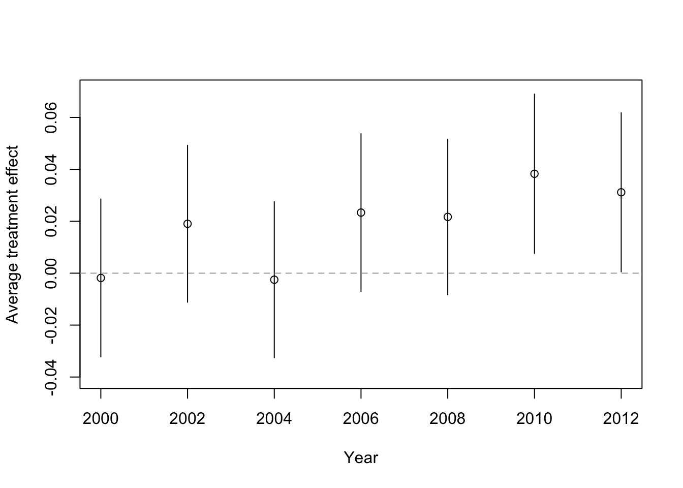
- Interpret the plot you have created.
Reveal answer
The plot simply visualises the difference in means and the confidence intervals that you created in question 4: it shows that the average treatment effect is positive in all years except for 2004, but also that the confidence intervals overlap with zero in all years except for 2010 and 2012 (we can see this from the fact the confidence intervals overlap the horizontal line you have added at 0 on the y-axis of the plot with the
abline()function).
8.3 Homework
The data for this weeks homework is the same as we used in the seminar.
In the seminar, we claimed that control group individuals are similar to treatment group individuals in all aspects except the treatment status (being a family member of a victim). This claim lays the foundation for the unconfoundedness assumption and allows us to use the difference in means as an estimate of the average treatment effect. To examine the validity of our claim, check whether possible confounders (observable characteristics) are balanced between the treatment and control groups. Specifically:
- Compare the difference in means (i.e., check the balance) for
fam.members,age,pct.white, andmedian.incomebetween the treatment and control groups. - For each of these comparisons, also calculate the respective 95% confidence intervals.
- Provide a brief interpretation of the results. What can you conclude about the potential for confounding (our unconfoundedness assumption) between the treatment and control groups?
Reveal answer
# Calculate the difference in means for family members
diff_fam_members <- mean(victims$fam.members[victims$treatment == 1]) -
                    mean(victims$fam.members[victims$treatment == 0])

diff_fam_members

# T-test for average family members in treatment and control
t_test_fam_members <- t.test(x = victims$fam.members[victims$treatment == 1],
                             y = victims$fam.members[victims$treatment == 0],
                             conf.level = 0.95)

t_test_fam_members$conf.int
## [1] -0.0598509
## [1] -0.14165792 0.02195612
## attr(,"conf.level")
## [1] 0.95# Calculate the difference in means for age
diff_age <- mean(victims$age[victims$treatment == 1]) -
mean(victims$age[victims$treatment == 0])
diff_age
# T-test for average age in treatment and control
t_test_age <- t.test(x = victims$age[victims$treatment == 1],
y = victims$age[victims$treatment == 0],
conf.level = 0.95)
t_test_age$conf.int## [1] -0.1607827
## [1] -1.0928107 0.7712453
## attr(,"conf.level")
## [1] 0.95# Calculate the difference in means for white voters
diff_pct.white <- mean(victims$pct.white[victims$treatment == 1]) -
mean(victims$pct.white[victims$treatment == 0])
diff_pct.white
# T-test for average proportion of white voters in treatment and control
t_test_pct.white <- t.test(x = victims$pct.white[victims$treatment == 1],
y = victims$pct.white[victims$treatment == 0],
conf.level = 0.95)
t_test_pct.white$conf.int## [1] 0.001567236
## [1] -0.01452926 0.01766374
## attr(,"conf.level")
## [1] 0.95# Calculate the difference in means for income
diff_median.income <- mean(victims$median.income[victims$treatment == 1]) -
mean(victims$median.income[victims$treatment == 0])
diff_median.income
# T-test for average income of voters in treatment and control
t_test_median.income <- t.test(x = victims$median.income[victims$treatment == 1],
y = victims$median.income[victims$treatment == 0],
conf.level = 0.95)
t_test_median.income$conf.int## [1] 522.727
## [1] -1487.766 2533.220
## attr(,"conf.level")
## [1] 0.95If treatment was “as-if” randomly assigned, the means on the three possible confounders should be similar across the two groups. While none of the point-estimates are exactly zero, the value of zero is included in each of the six confidence intervals. That means that, at the 95% confidence level, we cannot be confident that the true population difference in means is not equal to zero. In other words, the magnitude of observed differences between them is consistent with what we would expect to see purely by chance. This suggests that confounding is not a concern here (at least for the observable confounders in the data).
Question 2 (difficult)
In this question, you will create a function to explore the central limit theorem.
Plot a histogram of the
pct.whitevariable using thehist()function. Describe the distribution of the variable.Use the
sample()function (see below) to sample 200 values from thepct.whitevariable, and store the output as an object calledpct_white_sample. Make sure that you setreplace = TRUEin the sample function.
The sample() function randomly samples values from a vector. For instance, if you have a vector named my_vector, you can sample 100 values from that vector with:
Where the x argument is the vector from which you would like to sample, the size argument says how many observations you would like to sample, and the replace argument says whether you would like to sample from the vector with or without replacement. Use this code to do the sampling described above.
What is the mean of the sampled values? How does it compare to the mean of the original variable?
- Create a function which can be used to repeat this sampling process by adapting the code below:
sample_pct_white <- function(){

  # Add code here which samples 200 values from the pct white variable and
  # stores the output as an object called tmp_sample

  # Add code here which calculates the mean of tmp_sample
}
Use the
replicate()function to repeat the sampling process 1000 times. Store the 1000 mean values in an object calledsampling_distribution. You can look at R’s help files (through?replicateorhelp(replicate)) to better understand how to use thereplicate()function.Create a histogram of the
sampling_distribution. What is the shape of the distribution? Why does the histogram take this distinctive shape?
Reveal answer
1
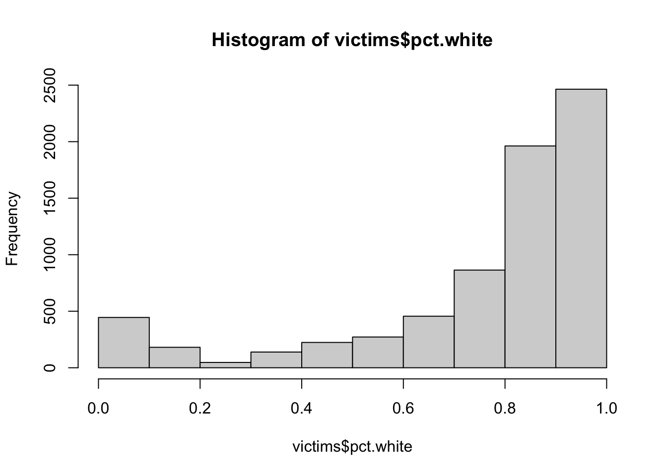
The distribution of the proportion of non-hispanic white voters living in the same block is quite left (negatively) skewed. This means that there are many more respondents who live in block with mainly white neighbours.
2
# Sample with replacement 200 values from the pct.white variable
pct_white_sample <- sample(victims$pct.white, 200, replace = TRUE)

# Calculate the mean of the sampled values
mean(pct_white_sample)

# Calculate the mean of all values
mean(victims$pct.white)
## [1] 0.742958
## [1] 0.7527122As the sampling is random, you might get a different sampled mean each time. Therefore, while it will nearly always be different from the mean of the original variable, it will sometimes be more, sometimes less different.
3
sample_pct_white <- function(){

  tmp_sample <- sample(victims$pct.white, 200, replace = TRUE)
  mean(tmp_sample)

}
4
# Replicate the sampling process 1000 times using function
sampling_distribution <- replicate(1000, sample_pct_white())
5
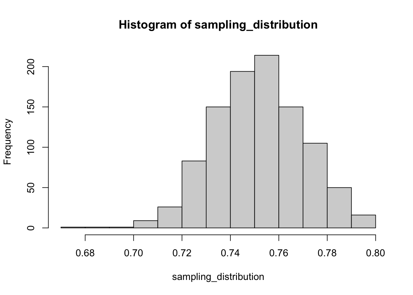
The distribution follows approximately a normal distribution. This is guaranteed by the central limit theorem, despite the fact that the underlying distribution of
pct_whiteis not normally distributed, so long as the sample size is large (here it is 200).