6 Regression III and Causality II
6.1 Overview
In the lecture this week, we discussed the use of regression for estimating causal effects. We saw that, when analysing data from randomized experiments, regression is a flexible tool that can help to a) understand treatment effect heterogeneity across different types of units; and b) calculate treatment effects for non-binary independent variables. We then discussed the assumptions required to make causal inferences from the analysis of observational data with regression models, and particularly focused on issues relating to omitted variable bias and “controlling” for confounding factors.
In the seminar this week, we will:
- Use regression as a method for “controlling” for potentially confounding covariates.
- Consider the assumptions required for making causal interpretations of regression coefficients.
- Practice calculating fitted values from an interaction model.
Before coming to the seminar, please read
Chapter 10 (except for the section “The Anatomy of a Regression”), in Bueno de Mesquita & Fowler (2021) Thinking Clearly with Data (essential)
Section 2.5.1, 2.5.2, and 4.3 (except for Section 4.3.4), in Quantitative Social Science: An Introduction (recommended)
6.2 Seminar
What is the monetary value of serving as an elected politician? Do politicians benefit financially because of their political offices? Chapter 4 of the textbook (pp. 176 - 181) reports on findings from a paper by Andrew Eggers and Jens Hainmueller (‘MPs for sale? Returns to Office in Postwar British Politics’) which investigates the financial returns to serving in parliament by studying data from the UK. Eggers and Hainmueller compare the wealth at the time of death for individuals who ran for office and won (MPs) to individuals who ran for office and lost (candidates) in order to draw causal inferences about the effects of political office on wealth. In this study, the margin of victory is used as a variable that creates “as if random” variation between election winners and election losers. The authors find that there is a large causal effect of holding office on wealth for Tory candidates, but a small causal effect of holding office for Labour candidates.
In this seminar, we will try to replicate these findings. We will use the same data, but rather than using the quasi-random variation induced by election results to identify the causal effect of office holding, we will instead use regression to control for potentially confounding variables.
The data set is in the csv file mps.csv, which you should download and store in your PUBL0055/data folder as in previous weeks. You should then make sure you working directory is set to the appropriate location, and then load the data as follows:
This data includes observations of 425 individuals. There are indicators for the main outcome of interest – the (log) wealth at the time of the individual’s death (ln.gross) – and for the treatment – whether the individual was elected to parliament (elected == 1) or failed to win their election (elected == 0). The data also includes information on a rich set of covariates.
The names and descriptions of variables are:
| Name | Description |
|---|---|
surname |
Surname of the candidate |
firstname |
First name of the candidate |
ln.gross |
Log gross wealth at the time of death |
ln.net |
Log net wealth at the time of death |
elected |
1 if the candidate was elected, 0 if they were not elected |
yob |
Year of birth |
yod |
Year of death |
aristo |
1 if the candidate had an aristocratic title of nobility, 0 otherwise |
female |
1 if the candidate is a woman, 0 otherwise |
region |
The region in which the candidate stood for election |
margin.pre |
Margin of the candidate’s party in the previous election |
margin |
Margin of victory (positive when the candidate won the election, negative when they lost the election) |
occupation |
The occupation of the candidate before they stood for election |
school |
The type of secondary school that the candidate attended |
university |
The type of university that the candidate attended |
party |
Whether the candidate stood for the Labour (“Labour”) or Conservative (“Tory”) party |
Question 1
Use a simple linear regression model to evaluate the relationship between gross wealth at death and whether or not a candidate was elected. Interpret the coefficient on the elected variable. Is the relationship positive or negative? Does this represent a causal difference?
Reveal answer
##
## Call:
## lm(formula = ln.gross ~ elected, data = mps)
##
## Residuals:
##     Min      1Q  Median      3Q     Max
## -3.9853 -0.4925 -0.0192  0.4244  3.5180
##
## Coefficients:
##             Estimate Std. Error t value Pr(>|t|)
## (Intercept) 12.41848    0.06466  192.07  < 2e-16 ***
## elected      0.51776    0.10377    4.99 8.85e-07 ***
## ---
## Signif. codes:  0 '***' 0.001 '**' 0.01 '*' 0.05 '.' 0.1 ' ' 1
##
## Residual standard error: 1.043 on 423 degrees of freedom
## Multiple R-squared:  0.05558,    Adjusted R-squared:  0.05335
## F-statistic:  24.9 on 1 and 423 DF,  p-value: 8.853e-07
The naive model suggests that politicians who are elected to parliament are 0.52 log points wealthier than politicians who were not elected to parliament. This is clearly not a causal difference, as there are many potentially confounding differences between those who are elected and those who are not elected. That is, it is likely that the difference estimated in this regression is subject to omitted variable bias.
Question 2
Create a box plot with
schoolon the x-axis andln.grosson the y-axis. Is there any association between the type of school attended by the candidate and the amount of money they were worth at the time of their death?What proportion of candidates who attended Eton were elected? What proportion of candidates who attended public school were elected? What proportion of candidates who attended “regular” schools were elected?
What do the results of the two subquestions above suggest about the relationship between gross wealth at death and whether a candidate was elected?
Estimate a new linear regression model to evaluate the relationship between gross wealth at death and whether or not a candidate was elected, but in this model you should also control for
school. Does the coefficient associated with theelectedvariable change when you include the additional control? Why?
Reveal answer
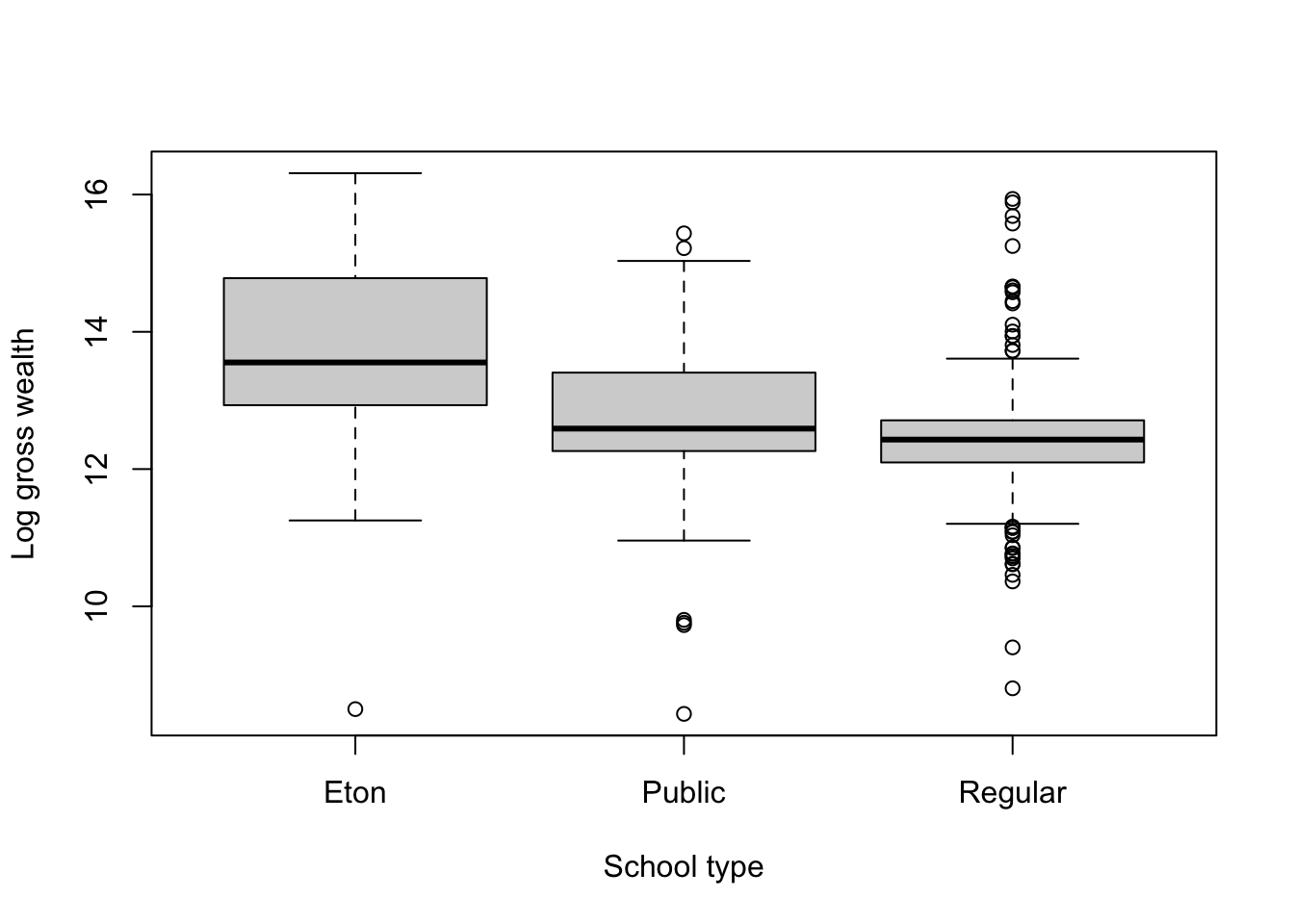
- Average wealth at the time of death clearly differs by the school that a politician attended. Those who attended Eton (a British “public” school which has been responsible for educating several UK Prime Ministers, as well as many MPs) are much wealthier on average at the time of their deaths than those from other “public” schools, or than those who attended “regular” schools.
##
##                   0         1
##   Eton    0.2222222 0.7777778
##   Public  0.6076923 0.3923077
##   Regular 0.6529851 0.3470149
- 78% of candidates who attended Eton were elected, compared to 39% from other public schools and 35% from regular schools.
- As we discussed in lecture, when dealing with observational data, we should always be wary about drawing causal conclusions from regression analyses because of the potential for confounding/omitted variable bias. The comparisons above show that the relationship between whether a candidate was elected and gross wealth at death is likely to be confounded by educational background.
In particular, omitted variables (variables not included in our regressions) will bias the regression estimates away from the causal effect of our explanatory variables when the omitted variable is correlated with both our independent variable and our dependent variable. In this example, there is a clear relationship between the type of school an individual attended and their wealth at death (as seen in the boxplot from question 2a). There is also a clear correlation between the type of school attended and whether the candidate won their election (as seen in the results from question 2b). Accordingly, both criteria for omitted variable bias are present here!
This implies that the regression coefficient from the
naive_modelthat we estimated in question 1 does not represent the causal effect of office holding on wealth, as it is subject to omitted variable bias.
control_model_1 <- lm(ln.gross ~ elected + school, data = mps)

library(texreg)
screenreg(list(naive_model, control_model_1))
##
## =====================================
## Model 1 Model 2
## -------------------------------------
## (Intercept) 12.42 *** 13.33 ***
## (0.06) (0.21)
## elected 0.52 *** 0.41 ***
## (0.10) (0.10)
## schoolPublic -0.75 ***
## (0.22)
## schoolRegular -1.02 ***
## (0.21)
## -------------------------------------
## R^2 0.06 0.11
## Adj. R^2 0.05 0.11
## Num. obs. 425 425
## =====================================
## *** p < 0.001; ** p < 0.01; * p < 0.05Controlling for
schoolleads to a decrease in theelectedcoefficient: it reduces from 0.52 in model 1 to 0.41 in model two. This change occurs because in the second model we are “holding constant” the school that the politician attended while estimating the effect of being elected to office on wealth.
Question 3
Examine the other variables in the data and select an additional three control variables to include in your model. Do not pick these at random, but rather think about whether there is reason to believe that these variables might be a cause of omitted variable bias in the model specification you estimated in question 2.
Does the coefficient on the
electedvariable change when you estimate your new model?Does the coefficient estimate associated with the
electedvariable now describe a causal effect? What assumptions are required to give this coefficient a causal interpretation? Can you think of any reasons why these assumptions may not be plausible in this context?
Reveal answer
control_model_2 <- lm(ln.gross ~ elected + school + aristo + female +
                        occupation, data = mps)

screenreg(control_model_2)
##
## ====================================
## Model 1
## ------------------------------------
## (Intercept) 13.50 ***
## (0.25)
## elected 0.42 ***
## (0.10)
## schoolPublic -0.86 ***
## (0.22)
## schoolRegular -1.05 ***
## (0.21)
## aristo 0.42
## (0.29)
## female 0.16
## (0.24)
## occupationjournalist -0.05
## (0.21)
## occupationlawyer 0.27
## (0.21)
## occupationlocal politics -0.13
## (0.20)
## occupationteacher -0.31
## (0.17)
## occupationunion -0.54
## (0.32)
## occupationwhite collar -0.10
## (0.21)
## ------------------------------------
## R^2 0.15
## Adj. R^2 0.13
## Num. obs. 425
## ====================================
## *** p < 0.001; ** p < 0.01; * p < 0.05
- We have estimated a model which includes three additional predictors –
aristo,femaleandoccupation– that are all plausibly associated with both the dependent variable and main independent variable in the analysis. Recall that omitted variable bias is a concern when we have reason to believe that the variables that are omitted are related both to X and Y.
In this case, it seems reasonable that whether a candidate is an aristocrat, whether they are female, and which occupation they had before running for office will all be correlated with whether or not the candidate wins the election (that is, they are probably correlated with X). Similarly, it seems likely that these factors are also correlated with the wealth of an individual when they die, and so are all potential sources of omitted variable bias.
##
## ============================================================
##                           Model 1     Model 2     Model 3
## ------------------------------------------------------------
## (Intercept)                12.42 ***   13.33 ***   13.50 ***
##                            (0.06)      (0.21)      (0.25)
## elected                     0.52 ***    0.41 ***    0.42 ***
##                            (0.10)      (0.10)      (0.10)
## schoolPublic                           -0.75 ***   -0.86 ***
##                                        (0.22)      (0.22)
## schoolRegular                          -1.02 ***   -1.05 ***
##                                        (0.21)      (0.21)
## aristo                                              0.42
##                                                    (0.29)
## female                                              0.16
##                                                    (0.24)
## occupationjournalist                               -0.05
##                                                    (0.21)
## occupationlawyer                                    0.27
##                                                    (0.21)
## occupationlocal politics                           -0.13
##                                                    (0.20)
## occupationteacher                                  -0.31
##                                                    (0.17)
## occupationunion                                    -0.54
##                                                    (0.32)
## occupationwhite collar                             -0.10
##                                                    (0.21)
## ------------------------------------------------------------
## R^2                         0.06        0.11        0.15
## Adj. R^2                    0.05        0.11        0.13
## Num. obs.                 425         425         425
## ============================================================
## *** p < 0.001; ** p < 0.01; * p < 0.05
- There is a small change in the estimated coefficient associated with the
electedvariable when controlling for these other factors, though it remains very similar to the coefficient that we estimated incontrol_model_1. This suggests that the school that a candidate attended is a larger source of omitted variable bias than the additional control variables that we added for this question.
- In order to interpret this coefficient as the causal effect of being elected, we have to assume that our regression model controls for all potentially confounding variables. While we have controlled for more variables in this specification than in either of the two previous models, is it fair to say that we have controlled for every possible omitted variable that might be the source of bias? Probably not.
For instance, one potential confounder that we are not controlling for is candidate quality – it may be the case that the people who are elected are just better in many ways that the people who are not elected. Those quality differences may also be correlated with lifetime earnings. As a consequence, our estimate of the effect of being elected would again be biased. This is a particularly difficult problem because it is not clear how we would go about measuring the quality of different candidates, as this is an essentially unobservable quantity! Accordingly, we should probably still be cautious about providing a causal interpretation of these results.
Question 4
The original paper from which this data is taken shows that the effect of serving in office (i.e. getting elected) on a candidate’s wealth is larger for Tory MPs than Labour MPs. In this question, you will adapt the regression specification that you selected in question 3c to allow the effect of elected to vary by party.
Estimate a new regression model which includes an interaction term between
electedandparty.Construct the fitted values for two Labour candidates (you may want to return to your code from seminar 4): one who was elected, and one who was not. Note that in order to calculate these values, you will have to choose values for all of the independent variables that you included in your model. Once you have calculated these values, exponentiate them using the
exp()function, which will convert them from the log scale into £ values. What is the effect, in pounds, of being elected as an MP for Labour candidates?Repeat the fitted values calculations above for Tory candidates. What is the effect, in pounds, of being elected as an MP for Tory candidates?
Reveal answer
interaction_model <- lm(ln.gross ~ elected * party + school + aristo +
                          female + occupation, data = mps)
screenreg(interaction_model)
##
## ====================================
## Model 1
## ------------------------------------
## (Intercept) 13.26 ***
## (0.28)
## elected 0.15
## (0.15)
## partyTory 0.07
## (0.13)
## schoolPublic -0.73 **
## (0.22)
## schoolRegular -0.87 ***
## (0.22)
## aristo 0.30
## (0.29)
## female 0.15
## (0.24)
## occupationjournalist 0.03
## (0.22)
## occupationlawyer 0.28
## (0.21)
## occupationlocal politics -0.05
## (0.20)
## occupationteacher -0.25
## (0.17)
## occupationunion -0.36
## (0.33)
## occupationwhite collar -0.07
## (0.21)
## elected:partyTory 0.43 *
## (0.21)
## ------------------------------------
## R^2 0.16
## Adj. R^2 0.14
## Num. obs. 425
## ====================================
## *** p < 0.001; ** p < 0.01; * p < 0.05# Select the covariate values at which to calculate predictions
# It is good practice to select the most common value for the additional
# covariates. For instance, attendance at "regular" schools is the most
# common response in our data, so we select that for school
labour_X_values <- data.frame(elected = c(0,1),
party = "Labour",
school= "Regular",
aristo = 0,
female = 0,
occupation = "white collar"
)
# Calculate the fitted values
labour_fitted_values <- predict(interaction_model,
newdata = labour_X_values)
# Exponentiate these values to convert them into pound amounts
exponentiated_lab_fitted_vals <- exp(labour_fitted_values)
# Calculate the difference in fitted values
lab_effect <- exponentiated_lab_fitted_vals[2] -
exponentiated_lab_fitted_vals[1]
- For a Labour candidate with these covariate values, we estimate that being elected increases wealth at the time of death by £36773.
# Select the covariate values at which to calculate predictions

tory_X_values <- data.frame(elected = c(0,1),
                            party = "Tory",
                            school= "Regular",
                            aristo = 0,
                            female = 0,
                            occupation = "white collar"
                            )

# Calculate the fitted values

tory_fitted_values <- predict(interaction_model, newdata = tory_X_values)

# Exponentiate these values to convert them into pound amount

exponentiated_tory_fitted_vals <- exp(tory_fitted_values)

# Calculate the difference in fitted values

tory_effect <- exponentiated_tory_fitted_vals[2] -
               exponentiated_tory_fitted_vals[1]
- For a Tory candidate, we estimate that being elected increases wealth at the time of death by £191378. This is therefore a much larger effect than for Labour Party candidates.
6.3 Homework
What explains support for insurgents during civil war? How can we measure support for insurgents? Chapter 3 of the textbook (pp. 75 - 122) reports on findings from a paper by Jason Lyall, Graeme Blair, and Kosuke Imai (‘Explaining Support for Combatants during Wartime: A Survey Experiment in Afghanistan’) which analyses a survey fielded in 2011 seeking to measure support for the Taliban in Afghanistan. In this homework, we will analyse the determinants of support for the Taliban using regression analysis.
NATO invaded Afghanistan in 2003 as part of a coalition of international troops named the International Security Assistance Force (ISAF). In an effort to “nation build” and defeat the Taliban, ISAF engaged in a “hearts and minds” campaign which combined economic assistance, service delivery, and protection in order to win the support of civilians. In this homework, we will analyse the effectiveness of ISAF’s campaign to win the “hearts and minds” of civilians in contested areas.
The data set is in the csv file afghan_data.csv, which you should download and store in your PUBL0055/data folder as in previous weeks. You should then make sure you working directory is set to the appropriate location, and then load the data as follows:
The dataset has been altered slightly for the purposes of this homework task. It includes 1097 respondents from areas that were identified by the ISAF as contested between government forces and the Taliban four months before the survey was fielded. The variables are:
| Name | Description |
|---|---|
district_id |
Each respondent is in a village and in a district. This is the unique identifier for the district. |
age |
Respondent’s age (in years). |
employed |
1 if respondents are employed, 0 if they are unemployed. |
educ.years |
Respondent’s years of education. |
income |
Respondent’s income level. There are five level, with low scores denoting low income. |
cerp_projects |
District-level variable which measures the total expenditure on ISAF Commander’s Emergency Response Program (CERP) short-term aid projects in 2010. |
sharia.courts |
1 if the district was home to a Taliban-run sharia court system, 0 otherwise. |
violence.count.taliban.5km |
The number of Taliban-initiated violent events within five kilometres of the village’s centre one year prior to the survey’s launch. |
violence.count.ISAF.5km |
The number of ISAF-initiated violent events within five kilometres of the village’s centre one year prior to the survey’s launch. |
treat.group |
The treatment group for the endorsement experiment: “control”, “taliban”, or “ISAF”. |
prison.reform |
See below. |
direct.elections |
See below. |
independent.election.commission |
See below. |
anti.corruption.reform |
See below. |
Survey experiments often involve randomly manipulated information presented to survey respondents. In this case, the authors employ endorsement experiments, where respondents are asked how much they support policies that are randomly endorsed by different actors. To read more about endorsement experiments, see point 5 on this website.
The endorsement experiments ask respondents their support for four policies: prison system reform (prison.reform); a proposal to allow Afghans to vote in direct elections when selecting leaders for district councils (direct.elections); reform of Afghanistan’s Independent Election Committee (IEC) (independent.election.commission); and finally, a proposal to strengthen a new anti-corruption institution (anti.corruption.reform). For more information on these reforms and why they were chosen, you can read pp.682-683 of their article.
For each question, respondents are randomly assigned to a control group in which no actor endorses the policy or a treatment group in which the Taliban or foreign forces (ISAF) endorse the policy. Therefore, differences between the control and treatment groups indicate the level of support for the actor that endorses the policy. Respondents were asked to indicate their level of support for the proposal on a are a 5-point scale: strongly agree (1), somewhat agree (2), indifferent (3), somewhat disagree (4), strongly disagree (5), don’t know (98), and refused to answer (99). The exact wording of all questions is:
Prison system reform: prison.reform
A recent proposal by the Taliban [or foreign forces] calls for the sweeping reform of the Afghan prison system, including the construction of new prisons in every district to help alleviate overcrowding in existing facilities. Though expensive, new programs for inmates would also be offered, and new judges and prosecutors would be trained. How do you feel about this proposal?
Direct Elections: direct.elections
It has recently been proposed by the Taliban [or foreign forces] to allow Afghans to vote in direct elections when selecting leaders for district councils. Provided for under Electoral Law, these direct elections would increase the transparency of local government as well as its responsiveness to the needs and priorities of the Afghan people. It would also permit local people to actively participate in local administration through voting and by advancing their own candidacy for office in these district councils. How do you feel about this proposal?
Independent Election Commission: independent.election.commission
A recent proposal calls by the Taliban [or foreign forces] for the strengthening of the Independent Election Commission (IEC). The Commission has a number of important functions, including monitoring presidential and parliamentary elections for fraud and verifying the identity of candidates for political office. Strengthening the IEC will increase the expense of elections and may delay the announcement of official winners but may also prevent corruption and election day problems. How do you feel about this proposal?
Anti-Corruption Reform: anti.corruption.reform
It has recently been proposed by the Taliban [or foreign forces] that the new Office of Oversight for Anti-Corruption, which leads investigations into corruption among government and military officials, be strengthened. Specifically, the Office’s staff should be increased and its ability to investigate suspected corruption at the highest levels, including among senior officials, should be improved by allowing the Office to collect its own information about suspected wrong-doing. How do you feel about this policy?
Responses to the endorsement questions were on a five point scale. However, “refuse to answer” and “don’t know” are coded as 98 and 99. NAs are often coded this way in surveys. If we do not recode these entries, they will affect our results. We cleaned the data using the ifelse() command:
afghan$direct.elections <- ifelse(           # If
  afghan$direct.elections.orig==98 |         # this statement ... or
    afghan$direct.elections.orig==99,        # ... this statement is true
  NA,                                        # then change it to this
  afghan$direct.elections.orig)              # but if not, then this

afghan$prison.reform <- ifelse(
  afghan$prison.reform.orig==98 | afghan$prison.reform.orig==99,
  NA,
  afghan$prison.reform.orig)

afghan$independent.election.commission <- ifelse(
  afghan$independent.election.commission.orig==98 |
    afghan$independent.election.commission.orig==99,
  NA,
  afghan$independent.election.commission.orig)

afghan$anti.corruption.reform <- ifelse(
  afghan$anti.corruption.reform.orig==98 |
    afghan$anti.corruption.reform.orig==99,
  NA,
  afghan$anti.corruption.reform.orig)
Question 1
Since the data have been recoded, solving the issue of “don’t know” and “refuse to answer”, please explore the variables for the endorsement experiment using the summary() or table() command.
Reveal answer
table(afghan$prison.reform)
table(afghan$direct.elections)
table(afghan$independent.election.commission)
table(afghan$anti.corruption.reform)
##
## 1 2 3 4 5
## 70 138 222 328 315
##
## 1 2 3 4 5
## 71 148 201 307 350
##
## 1 2 3 4 5
## 68 173 245 265 309
##
## 1 2 3 4 5
## 40 131 190 286 430Question 2
The authors ask several endorsement questions to avoid capturing the “idiosyncratic noise associated with a particular question” (p. 688). In their analysis, they pool the results of the endorsement experiments. We will do something similar by creating a variable for the mean response to the endorsement questions per individual. We will use a new function: rowMeans(). As always when you use a new function, check out how it works by typing ?rowMeans() in your console.
For this example, the code will take the following generic form:
We assign the mean value for three variables (var1, var2, and var3) to a new variable in our dataframe called new_variable. By setting the na.rm argument to TRUE, we ignore missing values when calculating the average response. For example, if a respondent only answered two endorsement questions, their average response will be the mean of these two values.
You can use this code to create your new variable.
- Create a new variable which is the average response of all four endorsement questions per respondent.
- Visualise your new variable as a function of the treatment groups. What does this indicate at first glance?
Reveal answer
afghan$endorsment_mean <- rowMeans(
  afghan[c("direct.elections", "prison.reform", "independent.election.commission", "anti.corruption.reform")],
                                   na.rm=TRUE)
As our new
endorsment_meanvariable is a continuous variable and our variable of interest is categorical, we can plot it as a boxplot.

The boxplot indicates that both treatments are slightly positive. If the endorsement question is capturing levels of support, it appears that support exists for both the ISAF and the Taliban in contest areas. Support for ISAF is generally higher.
Question 3
Analyse the effect of the endorsements (treat.group) on the average response created for Question 2.2. using linear regression. First analyse the effect on the newly created variable (endorsment_mean) and then analyse the effect on each endorsement question individually. Show your results in a two tables.
What do we learn about support for the ISAF and the Taliban in the areas surveyed? Looking at the endorsement questions individually, are you concerned?
Reveal answer
As the treatment is randomly assigned and the dependent variable is continuous , we can simply run a linear regression where the treatment group is a binary independent variable.
m1 <- lm(endorsment_mean ~ treat.group, data = afghan)

m2 <- lm(direct.elections ~ treat.group, data = afghan)

m3<- lm(prison.reform ~ treat.group, data = afghan)

m4 <- lm(independent.election.commission ~ treat.group, data = afghan)

m5 <- lm(anti.corruption.reform ~ treat.group, data = afghan)


screenreg(list("Average support" = m1))
##
## ===================================
## Average support
## -----------------------------------
## (Intercept) 3.89 ***
## (0.05)
## treat.groupISAF -0.54 ***
## (0.07)
## treat.grouptaliban -0.14 *
## (0.07)
## -----------------------------------
## R^2 0.06
## Adj. R^2 0.06
## Num. obs. 1090
## ===================================
## *** p < 0.001; ** p < 0.01; * p < 0.05The regression analysis reflects our interpretation of the boxplot for question 2. There appears to be support for both the Taliban and the ISAF. Support for the ISAF is stronger (-0.54) compared to the Taliban (-0.14). As the scale is 1 equals high support and 5 equals low support, a negative coefficient shows an increase in support.
##
## =============================================================================
##                     Direct elections  Prison       IEC          anti-corrupt.
## -----------------------------------------------------------------------------
## (Intercept)            3.93 ***          3.86 ***     3.70 ***     4.11 ***
##                       (0.07)            (0.06)       (0.07)       (0.06)
## treat.groupISAF       -0.33 ***         -0.59 ***    -0.43 ***    -0.73 ***
##                       (0.09)            (0.09)       (0.09)       (0.08)
## treat.grouptaliban    -0.46 ***         -0.10        -0.03         0.01
##                       (0.09)            (0.09)       (0.09)       (0.08)
## -----------------------------------------------------------------------------
## R^2                    0.02              0.04         0.03         0.09
## Adj. R^2               0.02              0.04         0.02         0.09
## Num. obs.           1077              1073         1060         1077
## =============================================================================
## *** p < 0.001; ** p < 0.01; * p < 0.05
It looks like the idiosyncrasies of the reform on direct elections might be driving our results for Taliban support, for which the coefficient (-0.46) is much higher than for other policy areas.
Question 4
Based on the results from previous questions, it is likely that there is support for both the ISAF and the Taliban in contested areas. Let’s think of ways in which the ISAF may increase support. We can assess treatment effect heterogeneity using interaction terms, where we interact our treatment variable (treat.group) with other variables of interest.
For a-c, show your results in both table and plot form. One of the goals of the ISAF was to win the “hearts and minds” of civilians:
One way of winning the hearts and minds is to provide greater funding for public goods provision. What is the effect of the endorsement experiment on respondents who live in districts with greater CERP short-term aid projects funding?
One way of losing the hearts and minds is by failing to prevent Taliban violence. What is the effect of the endorsement experiment on respondents who live in districts affected by Taliban violence?
Are you puzzled by these findings? Think about potential confounding when analysing your results.
Reveal answer
- Interact the treatment groups with two variables in order to assess heterogeneous levels of support in contested areas. The intuition is that some respondents live in areas where the “hearts and minds” campaign by the ISAF has been successful.
##
## =============================================
##                                   Model 1
## ---------------------------------------------
## (Intercept)                          4.23 ***
##                                     (0.07)
## treat.groupISAF                     -0.48 ***
##                                     (0.10)
## treat.grouptaliban                  -0.25 *
##                                     (0.10)
## cerp_projects                       -0.00 ***
##                                     (0.00)
## treat.groupISAF:cerp_projects       -0.00
##                                     (0.00)
## treat.grouptaliban:cerp_projects     0.00
##                                     (0.00)
## ---------------------------------------------
## R^2                                  0.15
## Adj. R^2                             0.14
## Num. obs.                         1090
## =============================================
## *** p < 0.001; ** p < 0.01; * p < 0.05
Support levels are generally higher among respondents who live in areas where there was more funding (as indicated by a negative coefficient for
cerp_projects). The slope is less negative (less supportive) for the Taliban treatment. This indicates that support increases especially for the ISAF.
The effect is more visible in Figure \(\ref{interaction1}\) below.
m7.isaf <- data.frame(cerp_projects =
                        c(0:max(afghan$cerp_projects)), treat.group="ISAF")
m7.taliban <- data.frame(cerp_projects =
                           c(0:max(afghan$cerp_projects)), treat.group="taliban")

pred.isaf <- predict(m7, newdata = m7.isaf)
pred.taliban <- predict(m7, newdata = m7.taliban)

plot(x = c(0:max(afghan$cerp_projects)),
     y = pred.isaf, type = "l", col = "blue",
     ylim = c(0, 5),
     xlab = "CERP projects",
     ylab = "Support")
lines(x = c(0:max(afghan$cerp_projects)),
      y = pred.taliban, lty = "dashed", col = "red")
text(100, 4.3, "Taliban\ntreatment", col = "red")
text(100, 3, "ISAF\ntreatment", col = "blue")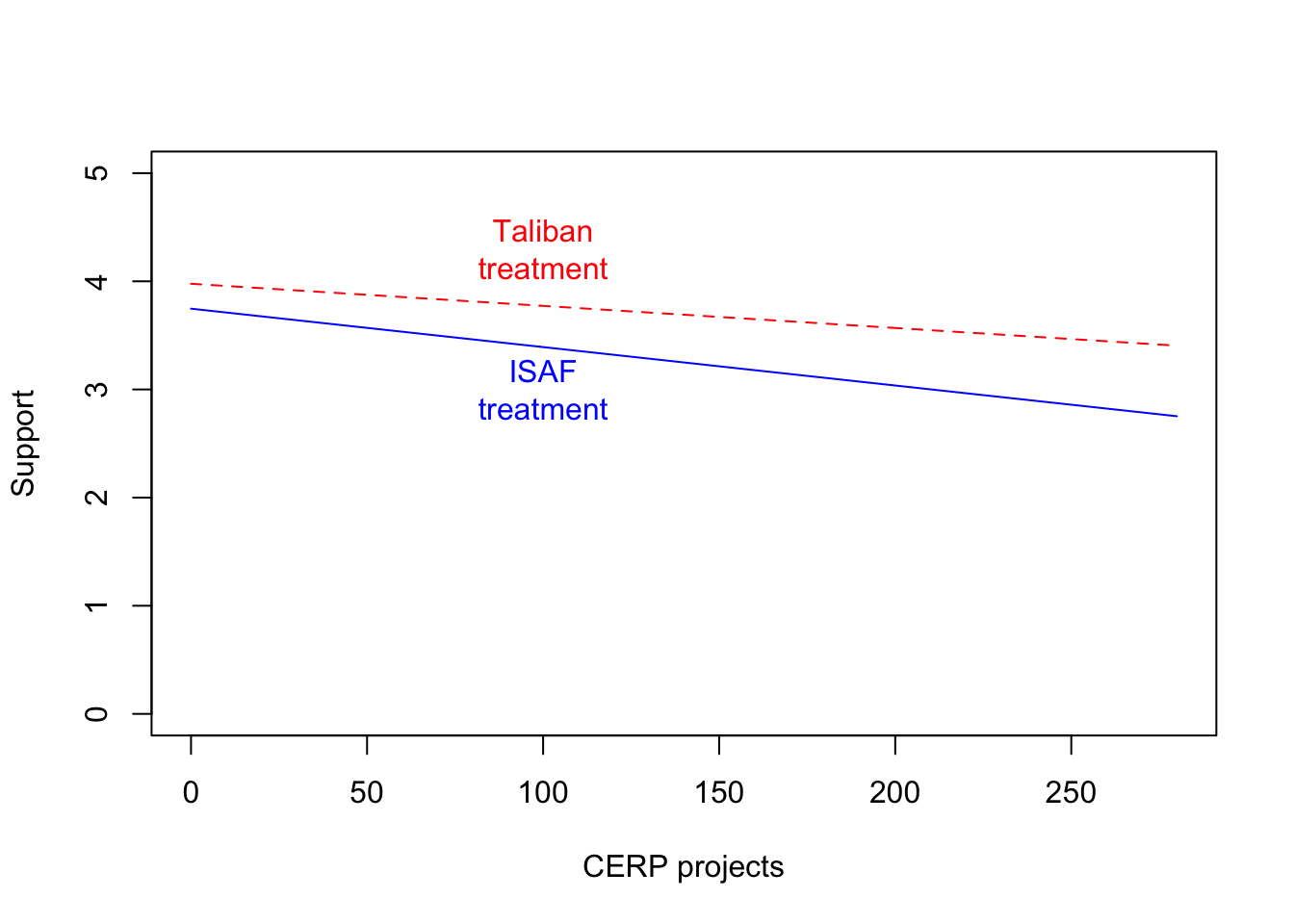
Figure 6.1: Answer 4.1.
##
## ==========================================================
##                                                Model 1
## ----------------------------------------------------------
## (Intercept)                                       3.99 ***
##                                                  (0.06)
## treat.groupISAF                                  -0.54 ***
##                                                  (0.09)
## treat.grouptaliban                               -0.27 **
##                                                  (0.09)
## violence.count.taliban.5km                       -0.00 *
##                                                  (0.00)
## treat.groupISAF:violence.count.taliban.5km        0.00
##                                                  (0.00)
## treat.grouptaliban:violence.count.taliban.5km     0.00 *
##                                                  (0.00)
## ----------------------------------------------------------
## R^2                                               0.07
## Adj. R^2                                          0.06
## Num. obs.                                      1090
## ==========================================================
## *** p < 0.001; ** p < 0.01; * p < 0.05
- Support levels are generally higher among respondents who live in areas where there were Taliban attacks (as indicated by a negative coefficient for
violence.count.taliban.5km). The slope is less negative (less supportive) for the Taliban treatment. This indicates that support increases for the ISAF in areas with more attacks.
The effect in Figure \(\ref{interaction1}\) below shows that Taliban attacks is associated with lower levels of support for the Taliban and higher levels of support for the ISAF. Areas with few attacks have similar levels of support.
m6.isaf <- data.frame(violence.count.taliban.5km =
                        c(0:max(afghan$violence.count.taliban.5km)), treat.group="ISAF")
m6.taliban <- data.frame(violence.count.taliban.5km =
                           c(0:max(afghan$violence.count.taliban.5km)), treat.group="taliban")

pred.isaf <- predict(m6, newdata = m6.isaf)
pred.taliban <- predict(m6, newdata = m6.taliban)

plot(x = c(0:max(afghan$violence.count.taliban.5km)),
     y = pred.isaf, type = "l", col = "blue",
     ylim = c(0, 5),
     xlab = "Count of taliban attacks",
     ylab = "Support")
lines(x = c(0:max(afghan$violence.count.taliban.5km)),
      y = pred.taliban, lty = "dashed", col = "red")
text(50, 4.3, "Taliban\ntreatment", col = "red")
text(50, 3, "ISAF\ntreatment", col = "blue")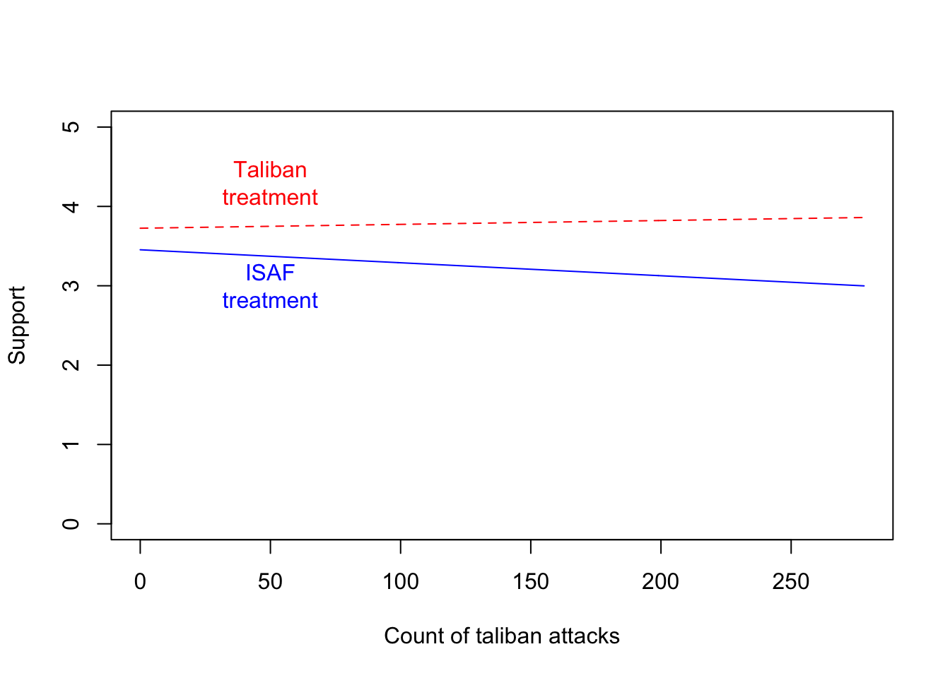
- Funding seems to increase ISAF support but also Taliban support. Taliban violence is associated with higher levels of support for the ISAF and slightly lower levels of Taliban support. This is counter-intuitive. It looks like the ISAF’s failure to protect districts from the Taliban may increase support for the ISAF. The Taliban might lose support in places where it conducts violence. Is the policy recommendation then to not protect communities from Taliban violence, in the hope that support for the ISAF will increase?
No! Key to understanding why we get these puzzling findings is that both funding and violence are not randomly assigned. Indeed, it is likely that the ISAF target areas where they want to win over support from those who support the Taliban, while the Taliban are more likely to attack places that support the ISAF.