9 Uncertainty II (Hypothesis testing)
9.1 Overview
In the lecture this week we continued our discussion of statistical inference, and particularly focussed on hypothesis tests and uncertainty in regression estimates. We learned about the different steps of conducting a hypothesis test, and about how to interpret both t-statistics and p-values. We saw the close connection between hypothesis tests and confidence intervals, and drew attention to the fact that observing a “statistically significant” result may not tell us anything about the substantive significance of that result. We also discussed uncertainty in regression models, and saw that our estimated regression coefficients are a quantity of interest that will vary from sample to sample, just as with the difference in means. Accordingly, we saw that we can also construct and interpret standard errors, t-statistics, p-values, and confidence intervals for our regression estimates.
In the seminar this week, we will:
- Practice conducting hypothesis tests for the difference in means.
- Practice conducting hypothesis tests for regression coefficients.
- Constructing confidence intervals for regression coefficients.
Before coming to seminar:
Please read Chapter 6, sections “Statistical Inference and Hypothesis Testing” until “Wrapping Up”, in Bueno de Mesquita & Fowler (2021) Thinking Clearly with Data (essential)
Please read Sections 7.2– 7.4, in in Quantitative Social Science: An Introduction (recommended)
9.2 Seminar
Are children of parents who are in same-sex relationships different from children of parents who are in heterosexual relationships? The New Family Structures Study (NFSS) sampled American young adults (aged 18-39) who were raised in various types of family arrangements. A sociologist, Mark Regnerus, published the debut article analysing data from the NFSS in 2012 and concluded that young adults raised by a parent who had a same-sex romantic relationship fared worse on a majority of 40 different outcomes, compared to six other family-of-origin types.
The controversial initial findings from the study were soon revisited and challenged by various scholars, including Cheng and Powell (2015) and Rosenfeld (2015). This controversy was at the heart of evidence presented in a Supreme Court case that struck down the Defense of Marriage Act and legalized gay marriage across the US. In 2015, the American Sociological Association filed an amicus brief with the Supreme Court stating that the initial study by Regnerus in 2012 “cannot be used to argue that children of same-sex parents fare worse than children of different-sex parents” because “the paper never actually studied children raised by same-sex parents.” This exercise is adapted from the initial study, along with two response papers:
Regnerus, Mark. 2012. “How different are the adult children of parents who have same-sex relationships? Findings from the New Family Structures Study.” Social Science Research, Vol. 41, pp. 752–770.
Cheng, Simon & Powell, Brian. 2015. “Measurement, methods, and divergent patterns: Reassessing the effects of same-sex parents.” Social Science Research, 52, pp. 615 - 626.
Rosenfeld, Michael J. 2015. “Revisiting the Data from the New Family Structure Study: Taking Family Instability into Account.” Sociological Science, 2, pp. 478-501.
To simplify the analysis, we focus on three mutually exclusive groups of household settings, used in the original study by Regnerus (we use the same names that Regnerus did in his original study). These are already coded and available in the data set: ibf if the respondent lived with mother and father from age 0 to 18 and their parents are still married at the time of the survey (referred to as “intact biological families”); lm if the respondent’s mother had a same-sex romantic relationship; gd if the respondent’s father had a same-sex romantic relationship; and other if the respondent belongs to neither the ibf nor same-sex families.
We focus mainly on two outcomes of interest: 1) level of depression of the respondent, measured by the CES-D depression index and 2) whether the respondent is currently on public assistance. The data set is the file nfss.csv. Download the data using the link above, save it into your data folder and load the data:
Variables in this data set are described below:
| Name | Description |
|---|---|
depression |
Scale ranges from 1-4 with higher numbers indicating more symptoms of |
| depression, as measured by the CES-D depression index | |
welfare |
1 if currently on public assistance, 0 otherwise |
ibf |
1 if lived in intact biological family, 0 otherwise |
lm |
1 if mother had a same-sex romantic relationship, 0 otherwise |
gd |
1 if father had a same-sex romantic relationship, 0 otherwise |
other |
1 if neither IBF nor had parents with same-sex relationship, 0 otherwise |
age |
Age in years |
female |
1 if female; 0 otherwise |
educ_m |
Mother’s education level: below hs (i.e., below highschool), hs, some college and |
college and above |
|
white |
1 if non-Hispanic white; 0 otherwise |
foo_income |
Respondent’s estimate of income of family-of-origin while growing up |
| (categorical variable with 7 income categories) | |
ytogether |
Number of years respondent lived with both parent and |
his/her same-sex partner; NA for respondents in ibf and other |
|
ftransition |
Number of childhood family transitions |
Question 1
We begin by comparing respondents in intact biological families (ibf) with those whose mother had a same-sex relationship (lm), as Regnerus did in his original study.
- What is the mean level of depression, respectively, for respondents in
ibfversuslmfamilies? Construct a 95% confidence interval around each estimate. Note that the depression measure is missing for some respondents, which need to be removed before computing its mean.
Reveal answer
# Calculate mean for ibf
mean.ibf <- mean(nfss$depression[nfss$ibf == 1], na.rm = TRUE)

## Standard error for ibf
var.ibf <- var(nfss$depression[nfss$ibf == 1], na.rm = TRUE)
n.ibf <- sum(nfss$ibf & !is.na(nfss$depression))
st_err_ibf <- sqrt(var.ibf / n.ibf)

# 95% confidence intervals for ibf

upper.ci.ibf <- mean.ibf + 1.96 * st_err_ibf
lower.ci.ibf <- mean.ibf - 1.96 * st_err_ibf
upper.ci.ibf
lower.ci.ibf

# Calculate mean for lm
mean.lm <- mean(nfss$depression[nfss$lm == 1], na.rm = TRUE)

## Standard error for lm
var.lm <- var(nfss$depression[nfss$lm == 1], na.rm = TRUE)
n.lm <- sum(nfss$lm & !is.na(nfss$depression))
st_err_lm <- sqrt(var.lm / n.lm)

# 95% confidence intervals for lm
upper.ci.lm <- mean.lm + 1.96 * st_err_lm
lower.ci.lm <- mean.lm - 1.96 * st_err_lm
upper.ci.lm
lower.ci.lm
## [1] 1.869881
## [1] 1.791707
## [1] 2.194379
## [1] 1.991038The mean level of depression for young adults in IBF is 1.83, with a standard error of 0.02. The 95% confidence interval is [1.79, 1.87]. The mean level of depression for young adults in LM families is 2.09, with a standard error of 0.05. The 95% confidence interval is [1.99, 2.19].
- We want to examine if young adults growing up in
lmfamilies have different levels of depression from those growing up inibf. Conduct a two-sided hypothesis test, using 5% as the significance level. Make sure to state your null hypothesis and alternative hypothesis explicitly.
Reveal answer
# Calculate the difference in means
diff.mean <- mean.lm - mean.ibf
diff.mean

# Standard errors
diff.se <- sqrt(st_err_lm ^ 2 + st_err_ibf ^ 2)
diff.se

# Calculate the t-test statistic
t_stat <- diff.mean/diff.se
t_stat

## T-test
t.test(nfss$depression[nfss$lm == 1], nfss$depression[nfss$ibf == 1])
## [1] 0.2619145
## [1] 0.05557394
## [1] 4.712902
##
## Welch Two Sample t-test
##
## data: nfss$depression[nfss$lm == 1] and nfss$depression[nfss$ibf == 1]
## t = 4.7129, df = 208.67, p-value = 4.458e-06
## alternative hypothesis: true difference in means is not equal to 0
## 95 percent confidence interval:
## 0.1523562 0.3714728
## sample estimates:
## mean of x mean of y
## 2.092708 1.830794Null hypothesis: There is no difference in average depression levels between young adults growing up in IBF and LM families. Alternative hypothesis: There is a difference in average depression levels between young adults growing up in IBF and LM families. The p-value is less than 0.05, therefore we reject the null hypothesis and conclude that there is a statistically significant difference in depression levels between young adults from IBF and LM families at the 5% significance level.
- Can we claim that having a mother who had a same-sex relationship causes young adult children to be more depressed? Why or why not?
Reveal answer
No. We cannot claim that the effect is causal because young adults from LM families and those from IBF families might differ in other ways that also affect their depression levels, such as family stability.
Question 2
Now we use regression models to estimate the difference in depression levels among young adults raised in different family arrangements.
- Run a linear regression to estimate the difference in depression level among respondents in the four groups (
lm,gd,ibf,other). Include the binary group variables in the regression as independent variables, and omitibfto make it the reference group. Based on the results from the regression: What is the estimated difference in depression level betweenlmandibf? How does it compare to your finding in Question 1.1? What is the estimated average depression level among those inibf? How does it compare to your finding in Question 1.1? What is the estimated average depression level among young adults ingd? Interpret each of the coefficients, standard errors, and 95% confidence intervals.
Reveal answer
## fit the regression model
fit1 <- lm(depression ~ lm + gd + other, data = nfss)
fit1

# examine the output
summary(fit1)

# confidence intervals
confint(fit1)
##
## Call:
## lm(formula = depression ~ lm + gd + other, data = nfss)
##
## Coefficients:
## (Intercept) lm gd other
## 1.8308 0.2619 0.3749 0.1282
##
##
## Call:
## lm(formula = depression ~ lm + gd + other, data = nfss)
##
## Residuals:
## Min 1Q Median 3Q Max
## -1.20573 -0.45904 -0.08404 0.41596 2.16921
##
## Coefficients:
## Estimate Std. Error t value Pr(>|t|)
## (Intercept) 1.83079 0.02081 87.989 < 2e-16 ***
## lm 0.26191 0.05358 4.888 1.07e-06 ***
## gd 0.37494 0.07699 4.870 1.17e-06 ***
## other 0.12825 0.02546 5.036 5.03e-07 ***
## ---
## Signif. codes: 0 '***' 0.001 '**' 0.01 '*' 0.05 '.' 0.1 ' ' 1
##
## Residual standard error: 0.6246 on 2938 degrees of freedom
## (46 observations deleted due to missingness)
## Multiple R-squared: 0.01715, Adjusted R-squared: 0.01615
## F-statistic: 17.09 on 3 and 2938 DF, p-value: 5.285e-11
##
## 2.5 % 97.5 %
## (Intercept) 1.78999571 1.8715919
## lm 0.15685440 0.3669746
## gd 0.22398676 0.5258944
## other 0.07831675 0.1781777Compared to young adults from IBF, those from LM families score 0.26 higher on the depression scale, same as part 1.1. Average depression level among young adults in IBF is 1.83, same as part 1.1. Those in “gd” types of families score 2.21.
Walking through each coefficient, the coefficient for
lmis 0.26, and the estimated standard error is 0.05. We can tell that this is statistically significant at the 95% confidence level by noting that the standard error is well less than half the coefficient magnitude, that the t-stat is well above 1.96 (4.89), or that the p-value is well below the 0.05 threshold (these things are equivalent).
Next, the coefficient for
gdis 0.37, and the estimated standard error is 0.08. We can tell that this is statistically significant at the 95% confidence level by noting that the standard error is well less than half the coefficient magnitude, that the t-stat is well above 1.96 (4.87), or that the p-value is well below the 0.05 threshold (these things are equivalent).
Finally, the coefficient for
otheris 0.13, and the estimated standard error is 0.03. We can tell that this is statistically significant at the 95% confidence level by noting that the standard error is well less than half the coefficient magnitude, that the t-stat is well above 1.96 (5.04), or that the p-value is well below the 0.05 threshold (these things are equivalent).
- Following Regnerus (2012), add several control variables to the regression model in 2.1, including age, gender, mother’s education, race (non-Hispanic white or not), and perceived family of origin income. Justify your choice of control variables. Interpret the coefficients on
lm,gdandotherin relation to the scale of the outcome variable. Present the two sets of results next to one another, and interpret the 95% confidence intervals and statistical significance for the estimated coefficients.
Reveal answer
fit2 <- lm(depression ~ lm + gd + other + age + female + white + educ_m +
             foo_income, data = nfss)

# display results
library(texreg)
screenreg(list(fit1, fit2))

# coefficients
summary(fit2)

# 95% confidence intervals
confint(fit2)
##
## =================================================
## Model 1 Model 2
## -------------------------------------------------
## (Intercept) 1.83 *** 2.30 ***
## (0.02) (0.08)
## lm 0.26 *** 0.15 *
## (0.05) (0.06)
## gd 0.37 *** 0.34 ***
## (0.08) (0.09)
## other 0.13 *** 0.05
## (0.03) (0.03)
## age -0.01 ***
## (0.00)
## female 0.09 **
## (0.03)
## white 0.04
## (0.03)
## educ_mcollege and above -0.08
## (0.05)
## educ_mhs -0.04
## (0.04)
## educ_msome college -0.07
## (0.04)
## foo_income100 to 150K -0.30 ***
## (0.07)
## foo_income150 to 200K -0.33 **
## (0.10)
## foo_income20 to 40K -0.12 **
## (0.04)
## foo_income40 to 75K -0.14 ***
## (0.04)
## foo_income75 to 100K -0.21 ***
## (0.05)
## foo_incomeAbove 200K -0.24 *
## (0.11)
## -------------------------------------------------
## R^2 0.02 0.06
## Adj. R^2 0.02 0.05
## Num. obs. 2942 2120
## =================================================
## *** p < 0.001; ** p < 0.01; * p < 0.05
##
## Call:
## lm(formula = depression ~ lm + gd + other + age + female + white +
## educ_m + foo_income, data = nfss)
##
## Residuals:
## Min 1Q Median 3Q Max
## -1.19266 -0.45319 -0.08944 0.37963 2.23417
##
## Coefficients:
## Estimate Std. Error t value Pr(>|t|)
## (Intercept) 2.29690 0.07885 29.131 < 2e-16 ***
## lm 0.15329 0.06137 2.498 0.012571 *
## gd 0.33552 0.09038 3.712 0.000211 ***
## other 0.04912 0.03027 1.623 0.104832
## age -0.01206 0.00213 -5.660 1.72e-08 ***
## female 0.08870 0.02843 3.120 0.001831 **
## white 0.03957 0.02914 1.358 0.174630
## educ_mcollege and above -0.08303 0.04727 -1.757 0.079114 .
## educ_mhs -0.03884 0.04394 -0.884 0.376795
## educ_msome college -0.07211 0.04326 -1.667 0.095676 .
## foo_income100 to 150K -0.29551 0.06691 -4.417 1.05e-05 ***
## foo_income150 to 200K -0.32832 0.10207 -3.217 0.001317 **
## foo_income20 to 40K -0.11808 0.03934 -3.001 0.002720 **
## foo_income40 to 75K -0.14462 0.04111 -3.518 0.000444 ***
## foo_income75 to 100K -0.20984 0.05202 -4.034 5.68e-05 ***
## foo_incomeAbove 200K -0.23566 0.11222 -2.100 0.035852 *
## ---
## Signif. codes: 0 '***' 0.001 '**' 0.01 '*' 0.05 '.' 0.1 ' ' 1
##
## Residual standard error: 0.6088 on 2104 degrees of freedom
## (868 observations deleted due to missingness)
## Multiple R-squared: 0.0569, Adjusted R-squared: 0.05018
## F-statistic: 8.463 on 15 and 2104 DF, p-value: < 2.2e-16
##
## 2.5 % 97.5 %
## (Intercept) 2.14227615 2.451527497
## lm 0.03293946 0.273641660
## gd 0.15827485 0.512769387
## other -0.01024740 0.108478802
## age -0.01623356 -0.007879047
## female 0.03295418 0.144453737
## white -0.01757444 0.096707869
## educ_mcollege and above -0.17572541 0.009660770
## educ_mhs -0.12500152 0.047322750
## educ_msome college -0.15694203 0.012724728
## foo_income100 to 150K -0.42672298 -0.164305959
## foo_income150 to 200K -0.52849040 -0.128144812
## foo_income20 to 40K -0.19523374 -0.040923313
## foo_income40 to 75K -0.22524219 -0.064006564
## foo_income75 to 100K -0.31185922 -0.107823750
## foo_incomeAbove 200K -0.45573724 -0.015583380We choose those variables that help us account for potential confounders. For example, age could be a confounder, because it could impact both the likelihood that the parents’ had a same-sex romantic relationship and the respondent’s level of depression.
Controlling for age, gender, mother’s education, race (non-Hispanic white or not), and perceived family of origin income, those in
lmfamilies have 0.15 higher depression level than those inibfon average; those ingdhave 0.33 higher level of depression thanibf; those inotherhave 0.05 higher level of depression thanibf. The coefficients are of smaller magnitude but still in same directions compared to part a. None of the coefficients are large given the outcome is on a 4 point scale. The coefficients are different because we have added other independent variables which may confound the relation between family types and depression, allowing us to better compare the differences across groups.
The coefficients indicate that higher socioeconomic status (as described by mother’s education and income) reduces depression. The coefficients for mother’s education are negative (with mothers with no high school as the reference group) and income coefficients are also negative (with 0 to 20k as the reference group). This indicates that increases in socioeconomic status as measured by these family background variables, are associated with a decrease in levels of depression. Additionally, all else equal, females are more depressed than males and white respondents are slightly more depressed than nonwhite respondents.
- What is the predicted depression level for a 28-year old, non-Hispanic white, male respondent growing up in
ibfand whose mother had “some college” education and whose perceived family-of-origin income is 40 to 75k? What about a person with the same characteristics but from anotherfamily group?
Reveal answer
## yhat = intercept + 28*beta_age + 1*beta_white + 1*beta_some_college + 1*beta_40to75K
y.hat <- 2.29690  + 28*(-0.01206) + 0.03957 + (-0.07211) + (-0.14462)
y.hat

## all else equal, "other" family group
y.hat.2 <- 2.29690  + 28*(-0.01206) + 0.03957 + (-0.07211) + (-0.14462) + 0.04912
y.hat.2
## [1] 1.78206
## [1] 1.83118The predicted level of depression is 1.7821 for the first and 1.8312 for the second.
Question 3
Regnerus describes the results of this study as showing that young adults “raised by” parents in same-sex relationships fare differently from other young adults. Cheng and Powell (2015) used calendar data that was included in the original NFSS study but not used in the Regnerus paper to examine how many years the young adults categorized in lm and gd groups actually lived with their parent and the parent’s same-sex partner from age 0 to 18. This information is recorded by the variable ytogether in the data set provided. Note: the variable is missing for young adults in ibf and other because they do not have a parent with a same-sex relationship.
- Create two histograms, one for
lmand the other forgd, to show the distribution ofytogetherfor each group. Make sure to set the bin width to 1 year. Interpret the histograms. Does your finding strengthen or weaken Regnerus’ claim that his results show that children raised by same-sex parents are different? Justify your answer.
Reveal answer
## 3.1
hist(nfss$ytogether[nfss$lm == 1],
freq = FALSE,
breaks = max(nfss$ytogether[nfss$lm == 1]),
     xlab = "years living together",
     ylab = "density", xlim = c(0, 18),
     ylim = c(0, 1), main = "LM")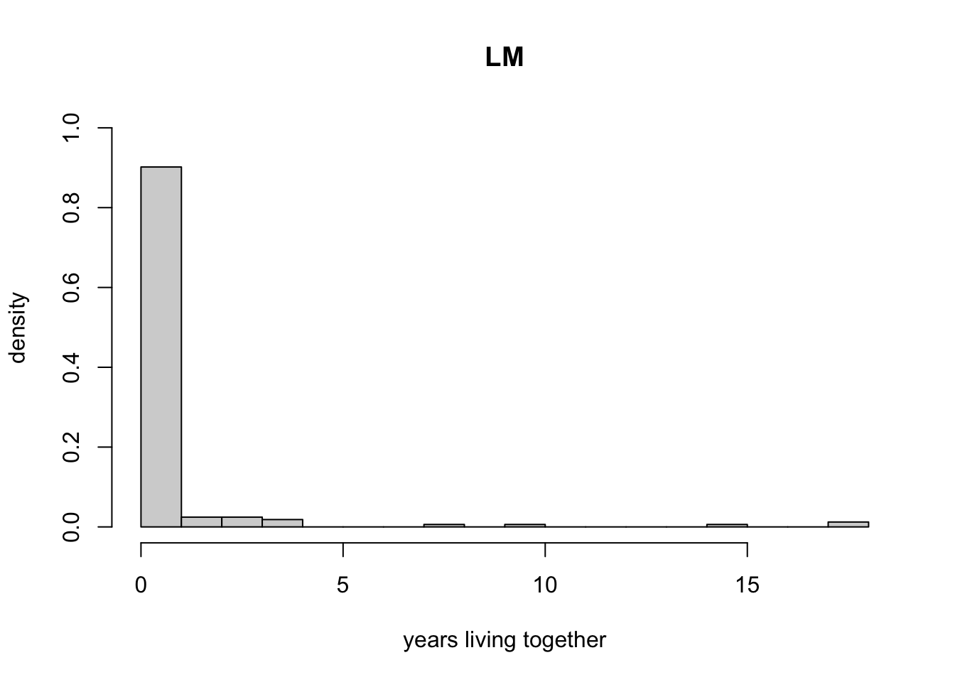
hist(nfss$ytogether[nfss$gd == 1],
freq = FALSE, breaks = max(nfss$ytogether[nfss$gd == 1]),
     xlab = "years living together",
     ylab = "density",xlim = c(0, 18),
     ylim = c(0, 1), main = "GD")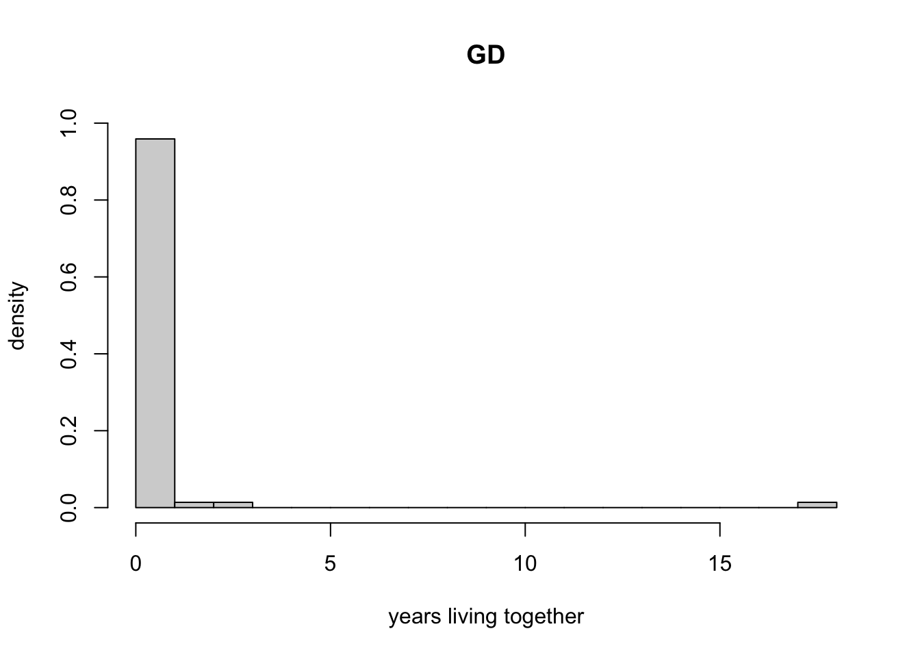
In both groups, the majority of respondents spent 0 years living with their the parents in same-sex partnerships. This calls into question that the categories defined by Regnerus were well suited for testing the hypothesis that being raised in these family structures has a negative impact on children.
- Do young adults in
lmfamilies who actually lived with the same-sex couple have different levels of depression from those growing up inibf? You will need to create a new variable (calledlm2, using theifelse()function), where you remove young adults who have never lived with their mother and her same-sex partner from thelmgroup. Then repeat the analysis in Question 1.2. Do your conclusions change?
Reveal answer
## create a new variable for same sex
nfss$lm2 <- ifelse(nfss$lm == 1 & nfss$ytogether > 0, 1, 0)

# Calculate mean for lm2
mean.lm2 <- mean(nfss$depression[nfss$lm2 == 1], na.rm = TRUE)

## Standard error for lm2
var.lm2 <- var(nfss$depression[nfss$lm2 == 1], na.rm = TRUE)
n.lm2 <- sum(nfss$lm2 & !is.na(nfss$depression))
st_err_lm2 <- sqrt(var.lm2 / n.lm2)

# 95% confidence intervals for lm2
upper.ci.lm2 <- mean.lm2 + 1.96 * st_err_lm2
lower.ci.lm2 <- mean.lm2 - 1.96 * st_err_lm2
upper.ci.lm2
lower.ci.lm2

# Difference in means
diff.means.2 <- mean.lm2 - mean.ibf

# Standard errors
diff.se2 <- sqrt(st_err_lm2 ^ 2 + st_err_ibf ^ 2)
diff.se2

# 95% confidence interval of diff in means
lower.ci.dim2 <- diff.means.2 - 1.96*diff.se2
upper.ci.dim2 <- diff.means.2 + 1.96*diff.se2
lower.ci.dim2
upper.ci.dim2

# t-statistic
t_stat.2 <- diff.means.2/diff.se2

## or t-test
t.test(nfss$depression[nfss$ibf == 1],nfss$depression[nfss$lm2 == 1])
## [1] 2.298358
## [1] 1.767118
## [1] 0.1369797
## [1] -0.06653595
## [1] 0.4704245
##
## Welch Two Sample t-test
##
## data: nfss$depression[nfss$ibf == 1] and nfss$depression[nfss$lm2 == 1]
## t = -1.4743, df = 26.094, p-value = 0.1524
## alternative hypothesis: true difference in means is not equal to 0
## 95 percent confidence interval:
## -0.48346066 0.07957213
## sample estimates:
## mean of x mean of y
## 1.830794 2.032738After removing those who have never lived with the parent and his/her single-sex partner, the difference is no longer statistically significant. Note that the confidence interval is slightly different when we calculate it by hand, but that’s nothing to worry about here.
Question 4
Rosenfeld (2015) challenged the findings from Regnerus by showing that family instability–adult household members moving into and out of the child’s household–explains most of the negative outcomes that had been attributed to same-sex parents. In the data set, we have included ftransition variable which was used by Rosenfeld to measure number of family transitions. For this question we will focus on a different outcome: the proportion of respondents on welfare.
- Create a new variable called
groupwhich includes different family groups (lm,gd,other,ibf). (Hint: you may want to revisit your code from seminar 5 if you do not remember how to create a new variable.)
Reveal answer
- Compute the mean number of family transitions (
ftransitions) for each group. Further examine the data by using boxplots. Describe your findings. According to your findings, do you think Intact Biological Families (ibf) is the best comparison group for studying the effect of having a parent who had same-sex relationship? Why or why not?
Reveal answer
## calculate the mean family transitions for each group
mean(nfss$ftransition[nfss$group=="lm"])
mean(nfss$ftransition[nfss$group=="gd"])
mean(nfss$ftransition[nfss$group=="ibf"])
mean(nfss$ftransition[nfss$group=="other"])

##  create boxplot
boxplot(ftransition ~ group, data = nfss,
        ylab = "Family transitions",
        main = "Family transitions by living arrangements")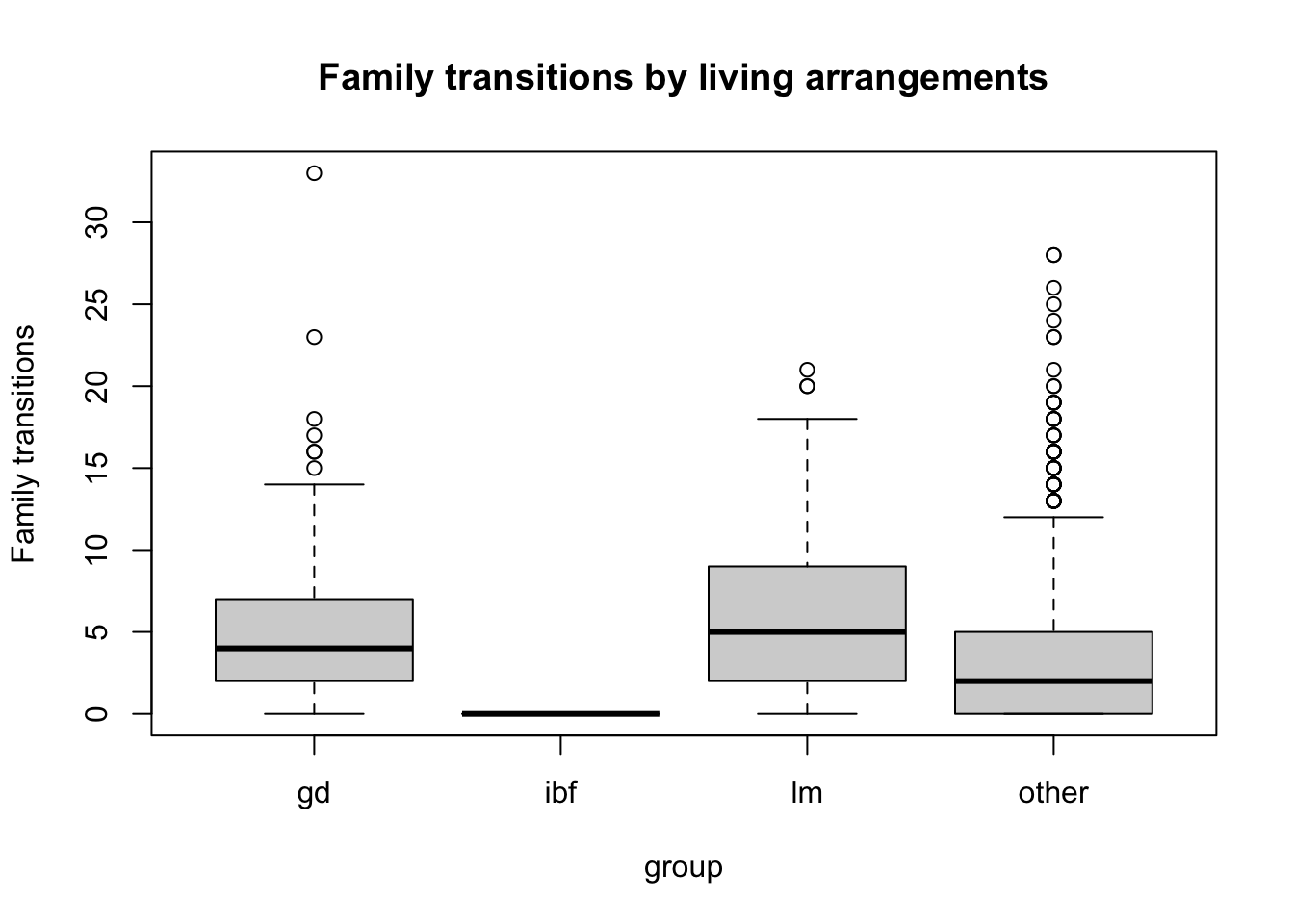
## [1] 6.429448
## [1] 5.767123
## [1] 0
## [1] 3.511184
The mean number of family transitions are 0 for IBF, 5.77 for GD, 6.43 for LM, and 3.51 for other families. The box plots show that the distribution of number of family transitions differs across the three groups: all the IBF are stable with 0 family transitions, whereas GD and LM families are not only much less stable on average, but the distribution of family transitions more dispersed.
IBF might not be a good comparison group because it differs from the same-sex families not only in the relationship of the parents but also family stability. Thus we cannot attribute all the differences we observe to parents’ relationship status only.