4 Regression (Prediction)
4.1 Overview
In the lecture this week, we discuss the simple linear regression model. We will introduce regression as a tool to explain associations between two continuous variables, and also as an alternative way of investigating the difference in means between groups. We will introduce the concept of model fit, and particularly focus on \(R^2\) as a statistic to summarise the predictive performance of our models.
In seminar this week, we will cover the following topics:
- The
lm()function. - The
predict()function. - Interpreting the output of simple linear regression models.
- Use of the
screenreg()command to nicely format simple regression models.
Before coming to the seminar
Please read:
Chapter 5 (“Regression for Describing and Forecasting”), sections “Regression Basics” and “The Problem of Overfitting”, in Bueno de Mesquita & Fowler (2021) Thinking Clearly with Data (essential)
Sections 4.1-4.2, in Quantitative Social Science: An Introduction (recommended)
4.1.1 Installing and loading packages
This week we will be using some additional functions that do not come preinstalled with R. There are many additional packages for R for many different types of quantitative analysis. Today we will be using the texreg package, which provides helpful functions for presenting the output of regression models.
To get started, you will need to install this packages on whatever computer you are using. Note: you only need to install a package on a computer once. Do not run this code every time you run your R script!
Once installed, you can load the packages using the library() function.
The general form of calling screenreg within the texreg package to create formatted regression tables is:
where we fit a simple regression model called model, with the dependent variable dependent and independent variable independent, from data dataset. We then run screenreg on the model object to display the formatted regression table.
Now you will be able to access the functions you need for the seminar and homework.
4.2 Seminar
What determines the electoral turnout rates of voters from ethnic minority groups? Existing theory suggests that one important driver of turnout for ethnic minority voters is when elections feature candidates from that ethnic group on the ballot paper. These candidate-centered approaches suggest that ethnic minority candidates may be better at, and devote more resources towards, mobilizing support from their co-ethnic electorates than other candidates. There is some empirical evidence that suggests that when a minority candidate is on the ballot, participation by minority voters increases.
An alternative theoretical perspective is that it is not the ethnicity of the candidate that matters, but rather the ethnic composition of the electorate. According to this view, when ethnic groups are a very small minority in a district, this implies a lack of descriptive representation which may produce a “disillusioned” electorate with little incentive to participate. If this is the case, then as the size of an ethnic group within a district increases, we should also expect increases in the rates of electoral participation for members of that ethnic group.
In a recent paper (“Candidates or Districts? Reevaluating the Role of Race in Voter Turnout”), Bernard Fraga evaluates both of these expectations using data from from US congressional and primary elections. We will use the data from this study to evaluate claims of this sort using regression analyses.
You can download the data from the link at the top of this page. Put the .csv into the your PUBL0055/data folder, and then load an R script to use this week. Don’t forget to set the working directory using the function setwd() as we have done for previous weeks.
Fraga analyzes turnout data for four different racial and ethnic groups, but for this analysis we will focus on the data for black voters. Load blackturnout.csv using the read.csv function.
A description of the variables is listed below:
| Name | Description |
|---|---|
year |
Year the election was held |
state |
State in which the election was held |
district |
District in which the election was held (unique within state but not across states) |
turnout |
The proportion of the black voting-age population in a district that votes in the general election |
CVAP |
The proportion of a district’s voting-age population that is black |
candidate |
Binary variable coded “1” when the election includes a black candidate; “0” when the election does not include a black candidate |
It will be a little easier to interpret the regression output if we convert the two proportion variables into percentages. Do this now using the following lines of code:
Question 1
Which years are included in the dataset? How many different states are included in the dataset?
For this question, try using two new functions that we have not introduced in previous weeks.
unique()returns the unique values of any particular vectorlength()returns the length of a vector, i.e. the number of observations in the vector
Reveal answer
## [1] 2008 2010 2006The
unique()function shows that there are three years included in the data: 2006, 2008 and 2010.
## [1] 42Wrapping the output of the
unique()function applied to the state variable in thelength()function reveals that there are 42 states in this data.
Question 2
In the following questions, we will be estimating several linear regression models. Linear regression is implemented in R using the lm() function. The lm() function needs to know a) the relationship we’re trying to model and b) the dataset that contains our observations. The two arguments we need to provide to the lm() function are described below.
| Argument | Description |
|---|---|
formula |
The formula describes the relationship between the dependent and independent variables, for example dependent.variable ~ independent.variable |
data |
This is simply the name of the dataset that contains the variable of interest. In our case, this is the merged dataset called blackturnout. |
For more information on how the lm() function works, type help(lm) in R.
a)
Create a scatter plot which has CVAP on the x-axis and turnout on the y-axis. Is the relationship between these variables positive or negative?
Reveal answer
plot(blackturnout$CVAP, blackturnout$turnout,
     xlab = "Black proportion of population",
     ylab = "Voter turnout (black voters)")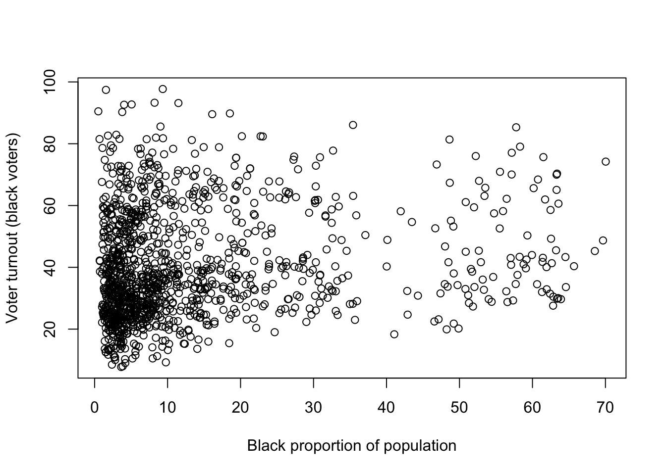
The relationship between the proportion of the population that is black, and the level of voter turnout among black voters is not terribly strong here, but the plot seems to reveal a moderate positive relationship.
b)
Estimate a linear regression model where the dependent variable is the percentage of the black people who voted in the election, and the independent variable is the percentage of a district’s voting-age population that is black. (Make sure that you get these the right way around!) Interpret the resulting \(\hat{\alpha}\) and \(\hat{\beta}\) coefficients.
Reveal answer
##
## Call:
## lm(formula = turnout ~ CVAP, data = blackturnout)
##
## Coefficients:
## (Intercept)         CVAP
##     37.5913       0.1957
The estimated \(\hat{\alpha}\) coefficient appears as the number associated with
(Intercept), and the \(\hat{\beta}\) coefficients appears as the number associated withCVAPin the regression output.
Recalling that \(\hat{\alpha}\) can be interpreted as the average value of \(Y\) when \(X = 0\), the intercept here suggests that the level of black turnout among districts with zero black voting-age individuals is equal to 37.6%. Is this a meaningful quantity? No - It doesn’t make much sense to speak of the turnout rate of black people in a place where no people are black! Furthermore, we can check the minimum value of the percentage of a district’s population that is black:
## [1] 0.5083851In this data, the district with the smallest share still has 0.5% of the voting-age population who are black. Accordingly, the intercept term here represents an extrapolation (though admittedly not a large one) outside of the range of the \(X\) variable in our data.
How about \(\hat{\beta}\)? The slope coefficient here is equal to 0.196, suggesting that a one-unit increase (a one percentage-point increase) in the percentage of a district’s population that is black is associated with an increase of approximately one-fifth of a percentage point in the turnout rate of black people, on average. This implies that there is indeed a positive relationship between the fraction of black people in a district’s population and the black turnout rate, at least in this data. In other words, in districts where black people make up a greater share of the voting-age population, black people in that district are more likely to vote in elections.
c)
Use the abline() function to add the estimated regression line to the scatter plot you created earlier. Read the help file for this function to see some different ways to achieve this.
Reveal answer
plot(blackturnout$CVAP, blackturnout$turnout,
     xlab = "Black proportion of population",
     ylab = "Voter turnout (black voters)")
abline(turnout_cvap_ols, col = "blue")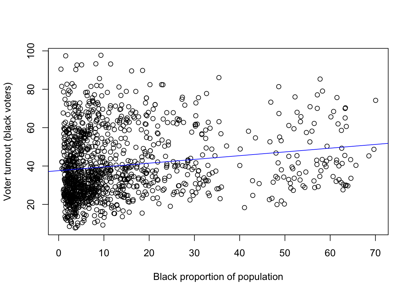
d)
Use the summary() function on your estimated linear regression model object. Also use screenreg to create a formatted regression table. Locate and interpret the \(R^2\) for this model.
Reveal answer
##
## Call:
## lm(formula = turnout ~ CVAP, data = blackturnout)
##
## Residuals:
##     Min      1Q  Median      3Q     Max
## -30.555 -12.760  -4.481  11.660  59.530
##
## Coefficients:
##             Estimate Std. Error t value Pr(>|t|)
## (Intercept) 37.59130    0.64050  58.690  < 2e-16 ***
## CVAP         0.19566    0.03254   6.012 2.41e-09 ***
## ---
## Signif. codes:  0 '***' 0.001 '**' 0.01 '*' 0.05 '.' 0.1 ' ' 1
##
## Residual standard error: 16.97 on 1235 degrees of freedom
## Multiple R-squared:  0.02844,    Adjusted R-squared:  0.02765
## F-statistic: 36.15 on 1 and 1235 DF,  p-value: 2.405e-09
The line that is second from bottom in the output reveals that the \(R^2\) in this case is 0.028. We can also use the
screenregcommand in thetexreglibrary to create a nicely formatted regression table:
##
## ========================
##              Model 1
## ------------------------
## (Intercept)    37.59 ***
##                (0.64)
## CVAP            0.20 ***
##                (0.03)
## ------------------------
## R^2             0.03
## Adj. R^2        0.03
## Num. obs.    1237
## ========================
## *** p < 0.001; ** p < 0.01; * p < 0.05
We can also directly extract the \(R^2\) from this model by using the
$operator at the end of the summary function:
## [1] 0.028437The \(R^2\) tells us the proportion of the variation in \(Y\) that is explained by the explanatory variable in our model. In this case, the \(R^2\) is relatively low, and implies that the percentage of a district’s population that is black explains only 2.8% of the variation in black voter turnout. This is obvious also from the plots we created above, where we can see that there is a lot of noise around the estimated regression line.
Question 3
Once we have estimated a regression model, we can use that model to produce fitted or predicted values. Fitted values represent our best guess for the value of our dependent variable for a specific value of our independent variable.
The fitted value formula is:
\[\hat{Y}_{i} = \hat{\alpha} + \hat{\beta} * X_i\]
Let’s say that, on the basis of turnout_cvap_ols we would like to know what percentage of the black population are likely to turnout in an election when the percentage of the district’s voting age population that is black is equal to 5%. We can substitute in the relevant coefficients from turnout_cvap_ols and the value for our X variable (5 in this case), and we get:
\[\hat{Y}_{i} = 37.59 + 0.196 * 5 = 38.57\]
Rather than calculating these values manually, we can also produce fitted values in R by using the predict() function. The predict function takes two main arguments.
| Argument | Description |
|---|---|
object |
The object is the model object that we would like to use to produce fitted values. Here, we would like to base the analysis on turnout_cvap_ols and so we specify object = turnout_cvap_ols. |
newdata |
This is an optional argument which we use to specify the values of our independent variable(s) that we would like fitted values for. If we leave this argument empty, R will automatically calculate fitted values for all of the observations in the data that we used to estimate the original model. If we include this argument, we need to provide a data.frame which has a variable with the same name as the independent variable in our model. Here, we specify newdata = data.frame(CVAP = 5), as we would like the fitted value for a district where 5% of the population is black. |
##        1
## 38.56958
This is the same as the result we obtained when we calculated the fitted value manually. The good thing about the predict() function, however, is that we will be able to use it for more complicated models that we will study later in this course, and it can be useful for calculating many different fitted values.
Calculate the predicted level of black turnout for two cases: where the percentage of black people in the population is equal to the 25th percentile and 75th percentile values for the distribution of that variable in the data. (That is, work out the fitted values for the interquartile range values of \(X\).)
Reveal answer
We can use the
quantile()function to find the relevant values of the explanatory variable:
##       25%       75%
##  3.520311 15.354315
Now we can pass the output of the
quantile()function to the predict function:
##        1        2
## 38.27610 40.60441
Evaluating these fitted values for the interquartile range of the \(X\) variable is another way of showing the substantive size of the association. In this case, we see that going from the 25th percentile value for \(X\) to the 75th percentile value for \(X\) increases the fitted or predicted value for \(Y\) by only about two percentage points. This suggests that the association between the proportion of black people in a district and the turnout rate among black people in a district is modest.
Question 4
a)
Create a boxplot that compares turnout in elections with and without a co-ethnic candidate. Be sure to use informative labels. Interpret the resulting graph. If you are struggling, look back at the code that we used last week to create boxplots.
(Note: the names argument of the boxplot function allows you to provide names for the groups which will appear under the relevant boxplot.)
Reveal answer
boxplot(turnout ~ candidate, data = blackturnout,
        names = c("Non-Coethnic Candidate", "Coethnic Candidate"),
        ylab = "Voter turnout (black voters)",
        xlab = "One or more co-ethnic candidates")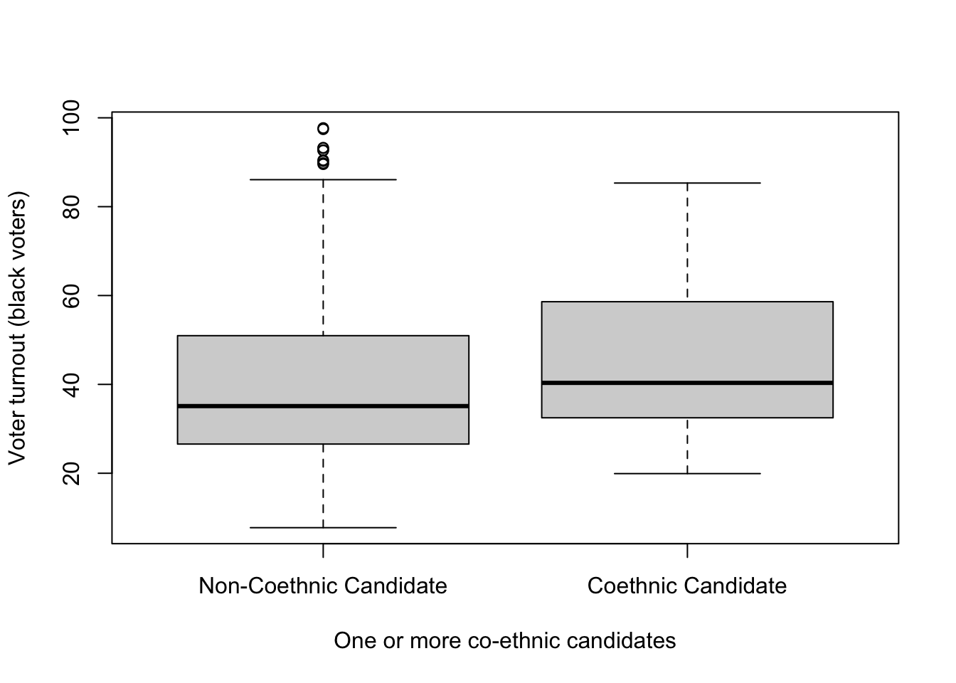
On average, it appears to be the case that black turnout tends to be higher when a co-ethnic candidate is running. We will come back to this relationship in more detail in the homework.
b)
At various point throughout this course it will be helpful if you can save the plots you have created as separate files so that they can be imported into documents that you are working on. In general, we recommend saving your plots as .pdf files.
The code below shows how to export a pdf of a plot directly to a folder on your computer. You should have a folder called PUBL0055, which currently contains your scripts and data. Create another subfolder and call it plots. You should then be able to save the plot you created above by using the following code:
Reveal answer
pdf("plots/coethnic_turnout_boxplot.pdf",8 ,8)
boxplot(turnout ~ candidate, data = blackturnout,
        names = c("Non-Coethnic Candidate", "Coethnic Candidate"),
        ylab = "Voter turnout (black voters)",
        xlab = "One or more co-ethnic candidates")
dev.off()
You will notice that nothing appears in the plotting window when you run this code, but if you have set up your folders correctly then a new plot called
coethnic_turnout_boxplot.pdfshould have appeared in theplotsfolder that you have just created.
Note that the
8, 8part of the code above tells R the dimensions of the image you would like to create (here you have specified that you would like a square plot which is 8 by 8 inches). You can try adjusting these numbers to see how they affect the shape of the image you are producing.
4.3 Homework
Question 1
Run a linear regression with black turnout as your dependent variable and candidate co-ethnicity as your independent variable. Remember to format your regression table using screenreg from the texreg package.
Reveal answer
turnout_candidate_ols <- lm(turnout ~ candidate, data = blackturnout)
screenreg(turnout_candidate_ols)
##
## ========================
## Model 1
## ------------------------
## (Intercept) 39.39 ***
## (0.52)
## candidate 6.16 ***
## (1.50)
## ------------------------
## R^2 0.01
## Adj. R^2 0.01
## Num. obs. 1237
## ========================
## *** p < 0.001; ** p < 0.01; * p < 0.05Question 2
Report the coefficient on your explanatory variable and also the intercept. Interpret these coefficients. Do not merely comment on the direction of the association (i.e., whether the slope is positive or negative). Explain what the value of the coefficients mean in terms of the units in which each variable is measured. Based on these coefficients, what would you conclude about black voter turnout and co-ethnic candidates?
Reveal answer
The intercept is 39.386 which means that in elections featuring no black candidates, approximately 39% of the black voting-age population are predicted to turn out. The coefficient on the candidate co-ethnicity variable is 6.164, which means that in elections with a black candidate black voter turnout is predicted to be about 6.2 percentage points higher on average. Thus, in elections featuring at least one black candidate, black voter turnout is predicted to be 45.55%. These results are consistent with the prediction that black voters turn out at a higher rate when a co-ethnic candidate is running.
Question 3
What is the relationship between the \(\hat{\beta}\) coefficient that you estimated in question 2 above and the difference in means?
Reveal answer
## Manual calculation of the difference in means
turnout_coethnic <- mean(blackturnout$turnout[blackturnout$candidate == 1])
turnout_noncoethnic <- mean(blackturnout$turnout[blackturnout$candidate == 0])

## Difference in means
turnout_coethnic - turnout_noncoethnic
## [1] 6.164014## candidate
## 6.164014As the manual calculation of the difference in means above suggests, the slope coefficient of the simple linear regression model when the independent variable is binary is equal to the difference in means that we have estimated in previous weeks. This will always be the case when we have a linear model with a single “dummy” explanatory variable, though not more generally when we include multiple explanatory variables in our models as we will see in future weeks.
Question 4
Does the estimate on the candidate variable above imply that there is a causal relationship between candidate ethnicity and black voter turnout? Why or why not?
Reveal answer
The estimated coefficient, or the equivalent difference in means, suggests that the presence of a black candidate is associated with higher levels of black turnout. In particular, districts in which a black candidate competes in the election have, on average, 6 percentage points higher levels of black turnout than districts without a black candidate.
Whether this difference reflects the causal effect of candidate ethnicity depends on whether we are confident in assuming that there is no other confounding bias between these types of districts. That is, we need to be confident that the only systematic difference between these districts is the presence or absence of a black candidate in the election. It seems implausible that this is true, as there are surely other factors that differ. For instance, as the analysis below shows, districts in which black candidates run also have a much higher percentage of the population in the district that is black.
Question 5
Use linear regression to assess the relationship between the proportion of a district’s population that is black (\(Y\)) and the presence of a black candidate (\(X\)). Interpret the estimates from your regression. What do these estimates suggest about the causal comparison you were asked to comment on in question 4?
Reveal answer
##
## Call:
## lm(formula = CVAP ~ candidate, data = blackturnout)
##
## Coefficients:
## (Intercept)    candidate
##        8.96        33.27
The regression implies that, on average, the black voting age population is 33 percentage points higher in districts that have a black candidate running in the election than the districts where no black candidate is running. More straightforwardly, this implies that black candidates often run in districts that have large black voting-age populations.
The upshot of this analysis is that it suggests that there may indeed be confounding bias in the relationship that we estimated in question 3, as we now know that districts with and without black candidates are indeed different with respect to (at least) this one variable. Accordingly, we cannot tell from these simple analyses whether the effect of black candidates on black turnout may in fact be attributable to the effects of the black composition of the district’s population.