7 Causality III (Observational data)
7.1 Overview
In the seminar this week, we will cover the following topics:
- Practice working with panel data.
- Calculating difference-in-differences using the
mean()function. - Calculating difference-in-differences using linear regression.
- Learning more about R’s plotting functions.
Before coming to the seminar, please read
Chapter 13, in Bueno de Mesquita & Fowler (2021) Thinking Clearly with Data (essential)
Sections 2.5.3 and 4.3.4, in Quantitative Social Science: An Introduction (recommended)
7.2 Seminar
The recent refugee crisis in Europe has coincided with a period of electoral politics in which right-wing extremist parties have performed well in many European countries. However, despite this aggregate level correlation, we have had (until a few years ago) surprisingly little causal evidence on the link between the arrival of refugees, and the attitudes and behaviour of native populations. What is the causal relationship between refugee protection crises and support for far-right political parties? Dinas. et al. (2018) examine evidence from the Greece. While some Greek islands (those close to the Turkish border) witnessed sudden and unexpected increases in the number of refugees during the summer of 2015, other nearby Greek islands experienced the arrival of way fewer refugees. In the paper, the authors use a difference-in-differences design to assess whether treated municipalities (i.e. those who receive high numbers of refugees) ended up with higher support for the far-right Golden Dawn party in the September 2015 General Election.
We will examine data from the paper, replicating the main parts of their difference-in-differences analysis. The exercise is based on Dinas, E., Matakos, K., Xefteris, D. and Hangartner, D., 2019. “Waking Up the Golden Dawn: Does Exposure to the Refugee Crisis Increase Support for Extreme-Right Parties?.” Political Analysis, Vol. 27, No. 2, pp. 244-254.
Up until now, almost all the data we have worked with on this course has been cross-sectional, which means that we have been working with one observation for each unit in our data. Whenever we have more than one observation in our data per unit, we can describe this data as having a panel structure. For instance in the exercises below, we will use the muni.Rdata file which contains data on 96 Greek municipalities (our units), and we observe the covariate and outcome variables for each municipality at multiple points in time (4 elections: 2012, 2013, 2015, and the post treatment year 2016).
Our goal in this exercise is to try and estimate causal relationships using observational data, panel data is therefore useful because we can make use of the fact that we observe variation in our main explanatory variables within units over time to rule out some forms of omitted variable bias. The muni.Rdata dataset that we will use this week is in panel data format, and contains the following variables:
| Name | Description |
|---|---|
municipality |
ID number for each municipality (factor) |
year |
Year of the election (numeric) – 2012; 2013; 2015; 2016 |
| ever_treated` | Binary – TRUE in all periods for all treated municipalities;
FALSE in all periods for all control municipalities |
post_treatment |
Binary – TRUE for all municipalities after treatment;
FALSE for all municipalities before treatment |
treatment |
Binary – 1 if the observation is in the treatment group
(a municipality that received refugees and the
observation is in 2016, the post-treatment period);
0 otherwise (untreated units and treated units in the
years 2012, 2013, 2015, the pre-treatment period) |
gdvote |
Continuous and the outcome of interest – Golden Dawn’s share of the vote |
The data can be download using the link above. Save the dataset to the same location on your computer as you have done in previous weeks, and then load it into an object called muni as below:
Question 1
Using only the observations from the post-treatment period (i.e. 2016), implement a regression which compares the Golden Dawn share of the vote for the treated and untreated municipalities. Does the coefficient on this regression represent a causal effect? If so, why? If not, why not?
Reveal answer
library(texreg)

# Subset the dataset to only the post-treatment period
post_treatment_data <- muni[muni$year==2016,]

# Estimate the linear regression model
post_treatment_period_regression <- lm(gdvote ~ treatment,
                                       data = post_treatment_data)

# Examine model
screenreg(post_treatment_period_regression)
##
## ======================
## Model 1
## ----------------------
## (Intercept) 5.66 ***
## (0.25)
## treatment 2.74 ***
## (0.71)
## ----------------------
## R^2 0.14
## Adj. R^2 0.13
## Num. obs. 96
## ======================
## *** p < 0.001; ** p < 0.01; * p < 0.05The
treatmentvariable is a dummy measuring1for treated observations in the post-treatment period, and zero otherwise. This means that the regression estimated above is simply the difference in means (for support for the Golden Dawn) between the treatment group (municipalities that witnessed large inflows of refugees) and the control group (municipalities that did not receive large numbers of refugees). The difference in means is positive: treated municipalities where on average 2-3 percentage points more supportive of the Golden Dawn than non-treated municipalities in the post-treatment period.
In order to be confident that this regression is estimating the causal effect of large inflows of refugees on Golden Dawn support, we would need to be confident that treated and control municipalities differ with respect to the influx of refugees only. However, because the treatment was not assigned at random, we cannot be confident in isolating this as the only systematic difference between treated and control municipalities. For instance, we currently cannot rule out that these municipalities might have always been more supportive of the Golden Dawn (perhaps they are poorer or have a different demographic make up which might influence their favourability towards the Golden Dawn). We therefore have little reason to believe that this difference in means would identify the causal effect of interest.
Question 2
Calculate the difference-in-differences between 2015 and 2016. For this question, you should calculate the relevant differences “manually”, in that you should use the mean() function to construct the appropriate comparisons. Use square brackets to subset the data. What does this calculation imply about the causal effect of the treatment on support for the Golden Dawn?
Note: Because the treatment variable only indicates differences in treatment status during the post-treatment period, you will need to use the ever_treated variable to define the difference in means in the pre-treatment period.
Reveal answer
# Calculate the difference in means between treatment and control
# in the POST-treatment period
post_difference <- mean(muni$gdvote[muni$ever_treated == TRUE & muni$year == 2016]) -
                   mean(muni$gdvote[muni$ever_treated == FALSE & muni$year == 2016])

# Difference in means in post-treatment
# Note that this is the same as we calculated above
post_difference

# Calculate the difference in means between treatment and control
# in the PRE-treatment period
pre_difference <- mean(muni$gdvote[muni$ever_treated == TRUE & muni$year == 2015]) -
                  mean(muni$gdvote[muni$ever_treated == FALSE & muni$year == 2015])

# Difference in means in pre-treatment
pre_difference

# Calculate the difference-in-differences
diff_in_diff <- post_difference - pre_difference

# Difference-in-differences
diff_in_diff
## [1] 2.744838
## [1] 0.6212737
## [1] 2.123564The difference in means in the post-treatment period (2.74) is larger than the difference in means for the pre-treatment period (0.62), implying that the average treatment effect on the treated municipalities is positive. In simple terms, the difference-in-differences implies that the refugee crisis increased support for the Golden Dawn amongst treated municipalities by roughly 2 percentage points, on average.
Question 3
Run a linear regression model to estimate the difference-in-differences. To this end, remember that you need to include in the regression
- a variable that accounts for the different treatment groups, i.e.
ever_treated; b.a variable that accounts for different treatment periods , i.e.post_treatment; and - a variable that accounts for whether a unit is actually treated, i.e.
treatment.
For this question, you should again focus only on the years 2015 and 2016. You can subset the data as such:
muni_1516 <- muni[muni$year >= 2015,]

# Note that this is equivalent to using the OR operator "|" as such:

muni_1516 <- muni[muni$year == 2015 |
                    muni$year == 2016, ]
Reveal answer
# Calculate the difference-in-differences
diff_in_diff_model <- lm(gdvote ~ ever_treated + post_treatment + treatment,
                        data = muni_1516)

screenreg(diff_in_diff_model)
##
## ==============================
## Model 1
## ------------------------------
## (Intercept) 4.39 ***
## (0.24)
## ever_treatedTRUE 0.62
## (0.68)
## post_treatmentTRUE 1.27 ***
## (0.34)
## treatment 2.12 *
## (0.97)
## ------------------------------
## R^2 0.18
## Adj. R^2 0.16
## Num. obs. 192
## ==============================
## *** p < 0.001; ** p < 0.01; * p < 0.05Recall our discussion of interaction effects from Week 5: the effect of the treatment (
ever_treated) on Golden Dawn vote support (gdvote) depends on whether we are looking in the pre- or post-treatment period (post_treatment). We see that the coefficient ontreatmentin the regression analysis gives us the same answer as the difference in differences in means we calculate in question 2: the estimated treatment effect for treated municipalities is an average of 2.12 percentage points higher vote share for Golden Dawn. Recall our discussion from the lecture that this is just another way of calculating the difference-in-differences. We will return to this next week, but regression has some advantages to the difference in means (namely: we get measures of uncertainty, such as the standard error and the p-value).
Question 4
In the lecture, we also used the interaction between treatment group and time period indicators to calculate the differences-in-differences. This is actually the same as using the treatment variable as we did in question 3. To investigate this further do the following:
- Create a new variable in the subsetted dataset where you interact (i.e. multiply)
ever_treatedandpost_treatment. Have a think about when the multiplication of these two dummies will be equal to 1 and when it will be equal to zero (Recall thatTRUEis treated equivalently to 1, andFALSEto 0 in calculations inR) - Compare this to the variable
treatmentusingtable(). What do you observe? - Run another regression, this time interacting
ever_treatedandpost_treatment. Compare this regression to the one from question 3. What do you observe?
Reveal answer
- The results of multiplying two variables with only FALSE (0) and TRUE (1) will only be equal to 1 where both variables are themselves equal to TRUE/1, as multiplying any number with FALSE/0 will always be zero. This means that the new variable will be 1 when
ever_treatedis TRUE andpost_treatmentis TRUE, i.e. for treated municipalities after treatment is applied.
##
##       0   1
##   0 180   0
##   1   0  12
- As we can see from cross-tabulating the two variables, they are identical.
# 3.
interaction_model <- lm(gdvote ~ ever_treated*post_treatment,
                        data = muni_1516)
screenreg(list(diff_in_diff_model,interaction_model))
##
## ===========================================================
## Model 1 Model 2
## -----------------------------------------------------------
## (Intercept) 4.39 *** 4.39 ***
## (0.24) (0.24)
## ever_treatedTRUE 0.62 0.62
## (0.68) (0.68)
## post_treatmentTRUE 1.27 *** 1.27 ***
## (0.34) (0.34)
## treatment 2.12 *
## (0.97)
## ever_treatedTRUE:post_treatmentTRUE 2.12 *
## (0.97)
## -----------------------------------------------------------
## R^2 0.18 0.18
## Adj. R^2 0.16 0.16
## Num. obs. 192 192
## ===========================================================
## *** p < 0.001; ** p < 0.01; * p < 0.05
- Once more, we see that the coefficient that we got from using
treatmentis identical to using the interaction betweenever_treatedandpost_treatment. This is becausetreatmentis equal to the multiplication/interaction of the treatment group and time period indicators. Note that sometimes it may be more convenient to use the interaction, especially if we want to calculate the treatment effect in each distinct time period. For instance, in this example, we may want to look at the difference between treatment and control at each election.
# first we need to convert year to a factor/categorical variable
muni$year2 <- as.factor(muni$year)

interaction_model2 <- lm(gdvote ~ ever_treated*year2,
                        data = muni)
screenreg(interaction_model2)
##
## ======================================
## Model 1
## --------------------------------------
## (Intercept) 5.49 ***
## (0.27)
## ever_treatedTRUE 0.67
## (0.78)
## year22013 -0.15
## (0.39)
## year22015 -1.11 **
## (0.39)
## year22016 0.17
## (0.39)
## ever_treatedTRUE:year22013 0.02
## (1.10)
## ever_treatedTRUE:year22015 -0.05
## (1.10)
## ever_treatedTRUE:year22016 2.08
## (1.10)
## --------------------------------------
## R^2 0.08
## Adj. R^2 0.07
## Num. obs. 384
## ======================================
## *** p < 0.001; ** p < 0.01; * p < 0.05This allows us to see the difference in each election before treatment. It would also be interesting to include election years after 2016 to investigate whether the effect remains or fades away.
Question 5
All difference-in-differences analyses rely on the “parallel trends” assumption. What does this assumption mean? What does it imply in this particular analyses?
Reveal answer
The parallel trends assumption requires us to believe that, in the absence of treatment, the treated and untreated units would have followed similar changes in the dependent variable. Another way of stating this assumption is that selection bias between treatment and control units must be stable over time (i.e. there can be no time varying confounders).
In this example, the assumption suggests that, in the absence of the large influx of refugees in the refugee crisis, treated and control municipalities would have experienced similar changes in the level of support for the Golden Dawn in the 2016 election.
Question 6
Assess the parallel trends assumption by plotting the evolution of the outcome variable for both the treatment and control observations over time. This means we need to look beyond the narrow window just before and just after treatment, and look also at the elections before 2015. Are you convinced that the parallel trends assumption is reasonable in this application?
Here we need to calculate the mean of the gdvote variable by both year and whether the unit was ever_treated. We could calculate each of these values manually and then store them in a data.frame for plotting, but this is likely to be very time consuming. Thankfully, there are a number of other ways to calculate the average outcome for treated and control units for each time period, and then to plot them on a graph. One solution is to use the aggregate() function which takes the following arguments:
| Argument | Description |
|---|---|
x |
The variable that you would like to aggregate. |
by |
The variable or variables that you would like to use to group the aggregation by. Must be included within the list() function. |
FUN |
The function that you would like to use in the aggregation (i.e. mean(), sum(), median(), etc.) |
Reveal answer
# Calculate the averages for year and ever_treated
group_period_averages <-
  aggregate(x = muni$gdvote, # Variable for which we want group means
  by = list(muni$year, muni$ever_treated), # We group by year and treatment
  FUN = mean) # Calculate mean for each group

# Add names to the variables
names(group_period_averages) <- c("year", "treated", "gdvote")

group_period_averages
## year treated gdvote
## 1 2012 FALSE 5.491237
## 2 2013 FALSE 5.339475
## 3 2015 FALSE 4.385363
## 4 2016 FALSE 5.659097
## 5 2012 TRUE 6.159583
## 6 2013 TRUE 6.023365
## 7 2015 TRUE 5.006637
## 8 2016 TRUE 8.403935There are many ways to plot the values you have estimated. You should use this question as a way of becoming familiar with the plot() function in R. Although you have used this function before, there are many options that you can specify to customise the graphics that you produce. I have provided a few below, and have made comments next to the code to aid understanding. I have also used the lines() function. This is similar to plot, and the main arguments it takes are an x and y vector.
plot(x = group_period_averages$year, # specifies variables plotted on the x-axis
     y = group_period_averages$gdvote, # specifies variables plotted on the y-axis
     col = ifelse(group_period_averages$treated==TRUE, "red", "blue"), # colour of points
     pch = 19, # determines the shape of the points on the plot
     xlab = "Year", # x-axis label
     ylab = "GD vote share", # y-axis label
     main = "Parellel trends?") # plot title

# Add a line to connect the estimated values over time for the treated units
lines(x = group_period_averages$year[group_period_averages$treated == TRUE],
      y = group_period_averages$gdvote[group_period_averages$treated == TRUE],
      col = "red")

# Add a line to connect the estimated values over time for the control units
lines(x = group_period_averages$year[group_period_averages$treated == FALSE],
      y = group_period_averages$gdvote[group_period_averages$treated == FALSE],
      col = "blue")

# Add vertical line to identify time of treatment
abline(v=2015.2)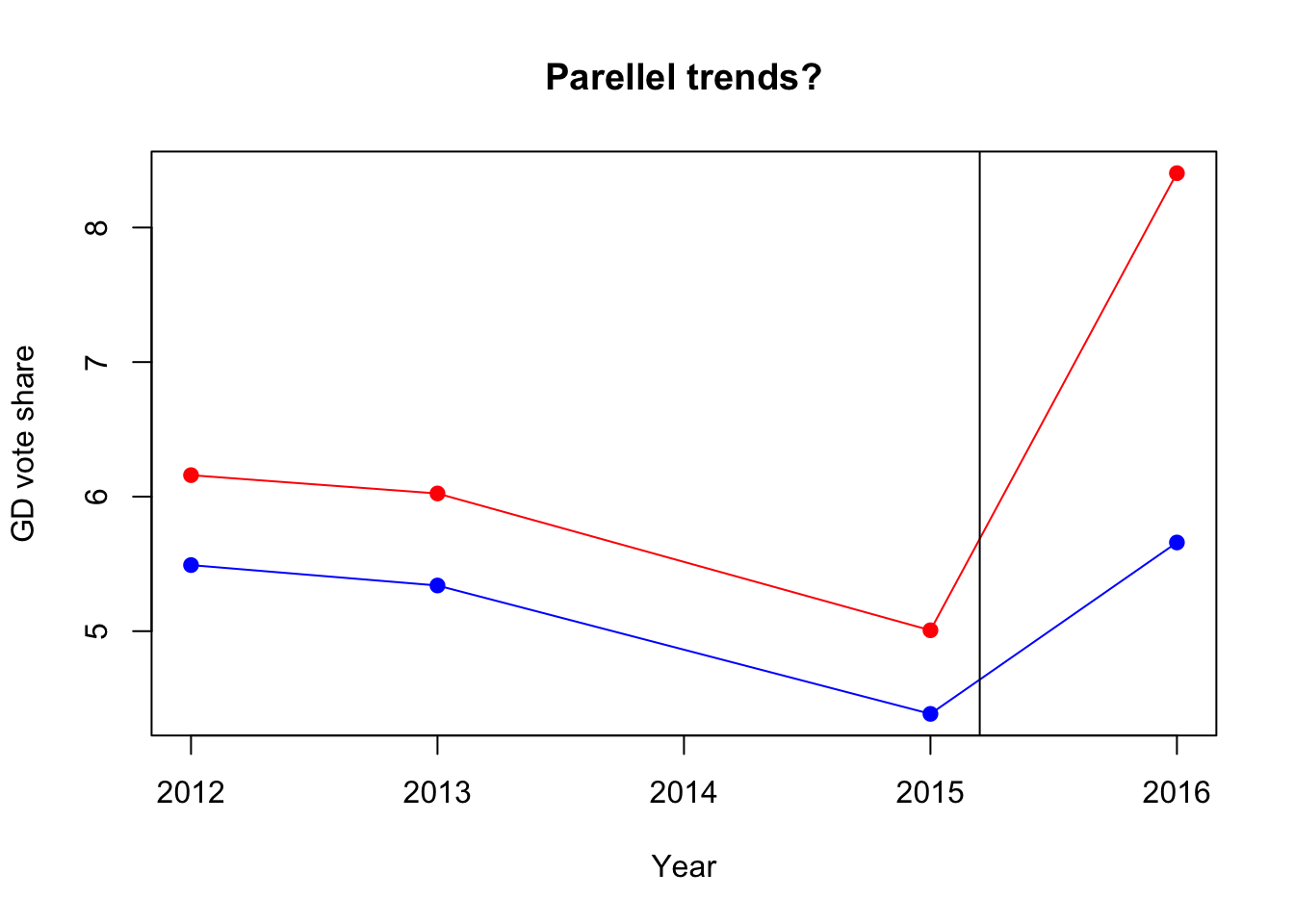
The plot reveals that the parallel trends assumption seems very reasonable in this application. The vote share for the Golden Dawn evolves in parallel for both the treated (red points) and control (blue points) municipalities throughout the three pre-treatment elections (2012, 2013, 2015), and then diverges noticeably in the post-treatment election (2016). This is encouraging, as it lends significant support to the crucial identifying assumption in this analysis.
7.3 Homework
In 2007, the Spanish government under the leadership of the PSOE (Spanish Socialist Worker’s Party) introduced the Law of Historical Memory which mandated municipalities to remove symbolic references to Francoist Spain between 1936 and 1975 in public spaces, including street names. In 2016, the first municipality was sentenced for not complying with the 2007 law. This prompted a larger number of municipalities to implement the law and remove Francoist street names in their territory. Focusing on municipalities that still had Francoist street names in June 2016, Villamil and Balcells (2021) examine if the VOX party, a radical right party in Spain founded in 2013, gained electorally from the removal of Francoist street names (in the 2019 elections). In this homework, you will explore whether the removal of Francoist street names after June 2016 increased support for VOX in elections in 2019.
The dataset street.csv is based on the original data by Villamil and Balcells (2021). You can download this data from the link above. Once you have done so, store it (without opening it otherwise) in your data subfolder and load it using the following code:
The names and descriptions of variables in the data set are:
| Name | Description |
|---|---|
muni_code |
Municipality code |
muni_name |
Municipality name |
pp |
Vote share PP (People’s Party) |
psoe |
Vote share PSOE (Socialist Workers’ Party) |
vox |
Vote share VOX |
left_major_2019 |
Leftist mayor in 2019 (0=no, 1=yes) |
unemp19 |
Unemployment rate (percentage) in 2019 |
lpop11 |
Log population (2011) |
treat |
Treatment - removed at least one Francoist street name (0=no, 1=yes) |
post |
Period (TRUE = June 2019, FALSE = June 2016) |
Question 1
How many municipalities are in the data set? (Hint: Remember this is panel data!)
What were the mean and median vote shares for the VOX party in 2016 and 2019, separately?
Visually inspect the distribution of the VOX vote share in 2016 and 2019.
Reveal answer
Answer 1.1
# We calculate the number of unique municipality codes in our data set
num_muni <- length(unique(streets$muni_code))
num_muni
## [1] 1169There are 1169 municipalities in the data set, which is far less than the 8135 municipalities in Spain. This is because the authors limit the analysis to municipalities where VOX ran in both 2016 and 2019, and which had at least one Francoist street name in 2016.
Answer 1.2
# There is more than one way to do this, but we can get all of the info from summary()
summary(streets$vox[streets$post==FALSE])
summary(streets$vox[streets$post==TRUE])
## Min. 1st Qu. Median Mean 3rd Qu. Max.
## 0.0000 0.0000 0.1379 0.2108 0.2681 5.0000
## Min. 1st Qu. Median Mean 3rd Qu. Max.
## 0.000 8.874 12.212 12.709 15.846 41.379In 2016, VOX’s median vote share in the municipalities included in the data set is 0.14 percent, and the mean vote share is 0.21 percent. In 2019, VOX’s median vote share in the municipalities included in the data set is 12.21 percent, and the mean vote share is 12.71 percent.
Answer 1.3
# There is more than one way to do this, but we can get all of the info from two histograms
par(mfrow=c(1,2))
hist(streets$vox[streets$post==FALSE], xlab="VOX vote share (2016)", main = "")
hist(streets$vox[streets$post==TRUE], xlab="VOX vote share (2019)", main = "")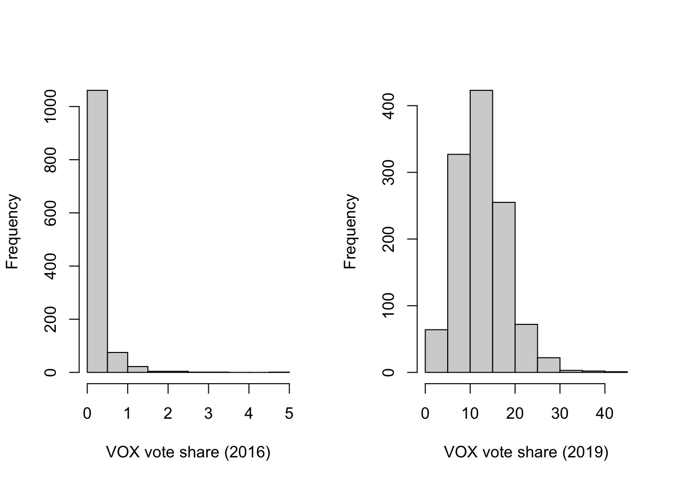
In 2016, VOX received less than 1 percent in the vast majority of municipalities, and did not gain more than 5 percent anywhere. The distribution of values is positively skewed. By contrast, VOX did much better across municipalities 1n 2019, receiving between 10 and 20 percent in many places.
Question 2
Is there an effect of removing Francoist street names on support for VOX?
- Start with the selection on observables design, using just the data on the 2019 elections—run a multiple linear regression and include all potential confounders. Justify your choice of control variables. (Hint: Use the subset of data where
postis TRUE.) - How confident are you that you can identify the causal effect using a selection on observables design here?
Reveal answer
Answer 2.1
# bivariate regression

m1 <- lm(vox ~ treat, data = streets[streets$post==TRUE,])
m2 <- lm(vox ~ treat + left_major_2019 + unemp19 + lpop11,
         data = streets[streets$post==TRUE,])
screenreg(list(m1,m2))
##
## =========================================
## Model 1 Model 2
## -----------------------------------------
## (Intercept) 12.54 *** 11.52 ***
## (0.18) (0.67)
## treat 0.74 0.72
## (0.38) (0.37)
## left_major_2019 -2.30 ***
## (0.32)
## unemp19 -0.03
## (0.06)
## lpop11 0.31 ***
## (0.09)
## -----------------------------------------
## R^2 0.00 0.05
## Adj. R^2 0.00 0.05
## Num. obs. 1169 1147
## =========================================
## *** p < 0.001; ** p < 0.01; * p < 0.05We need to think how each of the control variables added in the second model is related both to removal of Francoist street names and VOX support. For example, places with leftist mayors will have lower levels of (right-wing) VOX support and are more likely to remove Francoist street names.
Answer 2.2
Not confident at all! It is very likely that municipalities that are more likely to adhere to the law and change street names are less likely to have a large VOX voter base.
Question 3
We may be aware that there are many potential ways in which municipalities that removed Francoist street names after the first municipality got sentenced in 2016 differ in relevant ways (e.g., politically, socially, and economically) from municipalities that did not remove such street names. Therefore, let’s just focus on municipalities that removed at least on Francoist street name between June 2016 and June 2019 and investigate whether the VOX vote share in these municipalities increased from 2016 to 2019.
What is the difference in means in VOX vote shares in the June 2016 and April 2019 election in municipalities that removed at least one Francoist street name?
What assumptions would we need to make to interpret this estimate as the average causal effect? Is this likely?
Reveal answer
Answer 3.1
# We can calculate the difference in means "by hand"

# Mean VOX vote share in 2016 in municipalities with removed Francoist street names
avg_vox_treated_2016 <- mean(streets$vox[streets$post==FALSE & streets$treat==1])

# Mean VOX vote share in 2019 in municipalities with removed Francoist street names
avg_vox_treated_2019 <- mean(streets$vox[streets$post==TRUE & streets$treat==1])

# Calculate the difference in means
avg_vox_treated_2019 - avg_vox_treated_2016

# OR: we can do the same calculation using linear regression
vox.mod.1 <- lm(vox~post,data=streets[streets$treat==1,])
screenreg(vox.mod.1)
## [1] 13.06915
##
## =======================
## Model 1
## -----------------------
## (Intercept) 0.21
## (0.26)
## postTRUE 13.07 ***
## (0.37)
## -----------------------
## R^2 0.70
## Adj. R^2 0.70
## Num. obs. 532
## =======================
## *** p < 0.001; ** p < 0.01; * p < 0.05Whether we calculate the difference in means “by hand” or using a simple linear regression, we find that the VOX vote share increased on average by 13.07 percentage points between the two elections in places that removed at least one Francoist street name. This is an extremely substantial change—remember, the highest VOX support in 2016 was 5% and most municipalities’ saw VOX support of less than 1% in 2016.
Answer 3.2
To interpret this result as causal, we need to assume that there is no time-varying confounding. In other words, in the absence of Francoist street names being changed, that there would have not been any other causes that would impact the average vote share. We know from the answers to Question 1 that this is not the case. VOX was a relatively newly formed, fringe party in 2016, and received very few votes on average. By contrast, the average performance across Spanish municipalities improved greatly for VOX in 2019, and not only in places that removed Francoist street names. It is very likely that the before-after design does not allow us to estimate the true causal effect of removing at least one Francoist street name.
Question 4
In our sample, however, we also have municipalities that did not remove any Francoist street names between 2016 and 2019. This allows us to use a difference-in-differences design (as the authors in the original paper do) to estimate the average causal effect of removing Francoist street names on average support for VOX.
Calculate the difference-in-differences estimate, both by using group means (“by hand”) and with a linear regression model. What do you find?
Under what assumptions can the difference-in-differences estimate be interpreted as causal?
Reveal answer
Answer 4.1
# We can calculate the difference in means "by hand"

# Mean VOX vote share in 2016 in municipalities with removed Francoist street names
avg_vox_treated_2016 <- mean(streets$vox[streets$post==FALSE & streets$treat==1])

# Mean VOX vote share in 2019 in municipalities with removed Francoist street names
avg_vox_treated_2019 <- mean(streets$vox[streets$post==TRUE & streets$treat==1])

# Calculate the difference in means
diff_treated <- avg_vox_treated_2019 - avg_vox_treated_2016

# Mean VOX vote share in 2016 in municipalities with removed Francoist street names
avg_vox_control_2016 <- mean(streets$vox[streets$post==FALSE & streets$treat==0])

# Mean VOX vote share in 2019 in municipalities with removed Francoist street names
avg_vox_control_2019 <- mean(streets$vox[streets$post==TRUE & streets$treat==0])

# Calculate the difference in means
diff_control <- avg_vox_control_2019 - avg_vox_control_2016

# difference-in-differences
diff_treated - diff_control

# OR: we can do the same calculation using linear regression
did.model.vox <- lm(vox~treat*post, data=streets)
screenreg(did.model.vox)
## [1] 0.7391035
##
## ===========================
## Model 1
## ---------------------------
## (Intercept) 0.21
## (0.13)
## treat 0.00
## (0.27)
## postTRUE 12.33 ***
## (0.18)
## treat:postTRUE 0.74
## (0.38)
## ---------------------------
## R^2 0.73
## Adj. R^2 0.73
## Num. obs. 2338
## ===========================
## *** p < 0.001; ** p < 0.01; * p < 0.05Whether we calculate it by hand or use the regression model, we find that the estimated average causal effect is 0.74 percentage points. This means that the average change in VOX vote share between 2016 and 2019 is 0.74 percentage points more in municipalities that removed Francoist street names compared with municipalities that did not. This suggests that removing Francoist street names had a positive impact on VOX support, or as the authors interpreted it, as a right-wing / nationalist backlash against the policy.
Answer 4.2
To assume that this estimate can be interpreted causally, we need to assume “parallel trends”. In other words, if the Francoist street names had not been removed in our “treated” municipalities, the change in VOX vote share would have mirrored that in places that did not remove Francoist street names. This also means that we assume that there were no other causes between 2016 and 2019 that impacted the VOX vote share in different ways between “treated” and “control” municipalities.
Question 5
The authors of the original study not only focused on the change in vote share for VOX, but also examined whether the policy of removing Francoist street names impacted on the support for the mainstream parties. PSOE is the main centre-left political party in Spain, and the law to remove Francoist symbols was passed while they were in government.
What was the mean and median vote share for PSOE in 2019 for the municipalities under study?
Calculate the difference-in-differences estimate for PSOE. What do you conclude?
Reveal answer
Answer 5.1
# There is more than one way to do this, but we can all of the info from summary()
summary(streets$psoe[streets$post==TRUE])
## Min. 1st Qu. Median Mean 3rd Qu. Max.
## 0.00 26.23 31.84 33.08 39.64 68.33We find that the average vote share for PSOE in 2019 was 33.08 percent, and the median was 31.84 percent.
Answer 5.2
# We can do the PSOE calculation using linear regression
did.model.psoe <- lm(psoe~treat*post, data=streets)
screenreg(did.model.psoe)
##
## ===========================
## Model 1
## ---------------------------
## (Intercept) 29.13 ***
## (0.35)
## treat -1.12
## (0.74)
## postTRUE 4.26 ***
## (0.50)
## treat:postTRUE -0.23
## (1.05)
## ---------------------------
## R^2 0.04
## Adj. R^2 0.04
## Num. obs. 2338
## ===========================
## *** p < 0.001; ** p < 0.01; * p < 0.05The difference-in-differences estimate of -0.23 tells us that there was a bigger decrease in average support for PSOE (by 0.23 percentage points) in municipalities where Francoist street names were removed compared with municipalities where they were not. However, from the calculation in the first part of the question, the difference-in-differences estimate translates to a decrease of 100*0.23/33.08, or around 0.7 percent in average support for PSOE.
Question 6
Finally, the authors examine the vote shares for PP, the main party on the ideological Right in Spain. We repeat the analysis for PP that we conducted for PSOE in Question 5.
What was the mean and median vote share for PP in 2019 for the municipalities under study?
Calculate the difference-in-differences estimate for PP. What do you conclude?
Reveal answer
Answer 6.1
# There is more than one way to do this, but we can all of the info from summary()
summary(streets$pp[streets$post==TRUE])
## Min. 1st Qu. Median Mean 3rd Qu. Max.
## 3.013 17.557 22.989 24.705 30.100 76.923The average PP vote share in 2019 is 24.71 percent, and the median vote share is 22.99 percent.
Answer 6.2
# We can do the PSOE calculation using linear regression
did.model.pp <- lm(pp~treat*post, data=streets)
screenreg(did.model.pp)
##
## ===========================
## Model 1
## ---------------------------
## (Intercept) 41.22 ***
## (0.37)
## treat 5.55 ***
## (0.78)
## postTRUE -17.39 ***
## (0.52)
## treat:postTRUE -1.70
## (1.10)
## ---------------------------
## R^2 0.40
## Adj. R^2 0.40
## Num. obs. 2338
## ===========================
## *** p < 0.001; ** p < 0.01; * p < 0.05The difference-in-differences estimate of -1.70 tells us that there was a bigger decrease in average support for PP (by 1.70 percentage points) in municipalities where Francoist street names were removed compared with municipalities where they were not.
From the calculation in the first part of the question, the difference-in-differences estimate translates to a decrease of 100*1.70/24.71, or around 6.9 percent in average support for PP. This is a non-negligible amount.
Although there was not a wholesale defection from PP to VOX, the authors conclude that the results show that there was a “backlash” whereby more right-wing supporters of PP went to VOX in response the removal of Francoist street names.