5 Regression II (Specification)
5.1 Overview
In the seminar this week, we will cover the following topics:
- Use of the
load()command to load data sets in .Rdata/.rda format. - Use of the
lm()command to fit multiple linear regression models in R. - Use of the
screenreg()andhtmlreg()commands to compare differently specified multiple regression models. - Interpretation of categorical variables and interactions between variables.
- \(R^2\) and adjusted \(R^2\)
Before coming to the seminar
Please read:
Section 4.3.2, in Quantitative Social Science: An Introduction (essential)
5.1.1 Installing and loading packages
Like last week, we will be using some additional functions that do not come pre-installed with R. There are many additional packages forR for many different types of quantitative analysis. Today we will be using the texreg package, which we have encountered last week. It provides helpful functions for presenting the output of regression models.
# only run the line below if you have not YET installed texreg
# install.packages("texreg") # uncomment to run
library(texreg)
We saw the general form of calling screenreg within the texreg package last week. This week, we want to create side-by-side formatted regression tables. The general way to do this is:
5.2 Seminar
5.2.1 Economic Explanations for Opposition to Immigration
Why do the majority of voters in the U.S. and other developed countries oppose increased immigration? According to the conventional wisdom and many economic theories, people simply do not want to face additional competition on the labour market (economic threat hypothesis). Nonetheless, most comprehensive empirical tests have failed to confirm this hypothesis and it appears that people often support policies that are against their personal economic interest. At the same time, there has been growing evidence that immigration attitudes are rather influenced by various deep-rooted ethnic and cultural stereotypes (cultural threat hypothesis). Given the prominence of workers’ economic concerns in the political discourse, how can these findings be reconciled?
This exercise is based in part on Malhotra, N., Margalit, Y. and Mo, C.H., 2013. “Economic Explanations for Opposition to Immigration: Distinguishing between Prevalence and Conditional Impact.” American Journal of Political Science, Vol. 38, No. 3, pp. 393-433. You can find the study here.
The authors argue that, while job competition is not a prevalent threat and therefore may not be detected by aggregating survey responses, its conditional impact in selected industries may be quite sizeable. To test their hypothesis, they conduct a unique survey of Americans’ attitudes toward H-1B visas. A plurality of H-1B visas in the US are granted to Indian immigrants, who are high skilled but ethnically distinct, which enables the authors to measure a specific skill set (high technology) that is threatened by a particular type of immigrant (H-1B visa holders). The data set immig.Rdata has the following variables:
| Name | Description |
|---|---|
age |
Age (in years) |
female |
1 indicates female; 0 indicates male |
employed |
1 indicates employed; 0 indicates unemployed |
nontech.whitcol |
1 indicates non-tech white-collar work (e.g., law) |
tech.whitcol |
1 indicates high-technology work |
h1bvis.supp |
Support for increasing H-1B visas (5-point scale, 0-1) |
group |
Categorical: tech if someone is employed in tech; whitecollar
if someone is employed in other “white-collar” jobs;
other if someone is employed in any other sector; unemployed if someone is unemployed |
The main outcome of interest is level of support for/opposition to immigration. There are many different ways in which this concept of interest is measured in the literature. In this application, it was measured through support for/opposition to increasing the number of H-1B visa (h1bvis.supp).
Specifically, it was measured as a following survey item: “Some people have proposed that the U.S. government should increase the number of H-1B visas, which are allowances for U.S. companies to hire workers from foreign countries to work in highly skilled occupations (such as engineering, computer programming, and high-technology). Do you think the U.S. should increase, decrease, or keep about the same number of H-1B visas?”
The response options were the following: 0 = “decrease a great deal”, 0.25 = “decrease a little”, 0.5 = “keep about the same”, 0.75 = “increase a little”, 1 = “increase a great deal”.
You can download the data from the link at the top of this page. Put the data file into the your PUBL0055/data folder, and then load an R script to use this week. Don’t forget to set the working directory using the function setwd() as we have done for previous weeks.
Note unlike previous weeks, the data this week is not in csv format but in Rdata format. Instead of using the read.csv() function we use the load() function. We can load the dataset using the code below:
Question 1
If the labour market hypothesis described above is correct, opposition to H-1B visas should be more pronounced among those who are economically threatened by this policy such as individuals in the high-technology sector. Regress H-1B visa support on the dummy variable for tech workers (tech.whitcol).
- Interpret the intercept and the coefficient of the independent variable.
- Do the results support the labour market hypothesis? Is opposition to H-1B visas more pronounced among those who are economically threatened by this policy such as individuals in the high-technology sector?
Reveal answer
##
## =========================
##               Model 1
## -------------------------
## (Intercept)      0.35 ***
##                 (0.01)
## tech.whitcol    -0.05
##                 (0.04)
## -------------------------
## R^2              0.00
## Adj. R^2         0.00
## Num. obs.     1122
## =========================
## *** p < 0.001; ** p < 0.01; * p < 0.05
Instead of using screenreg to print the results on screen, we can save the formatted regression table into a Word file with the command (saved in a file called immig_lmfit1.doc):
The intercept tells us that the average support for H-1B visas among non-white collar tech workers is 0.35. The coefficient tells us that those who work in white collar tech jobs are slightly less supportive, specifically by about -0.05 on average. It is worth noting though that the effect is quite small in substantive terms.
Overall, the results provide some support for the labor market hypothesis: those who are in sectors in which H-1B visa holders are more likely to work in (and therefore are more economically threatened) are less supportive of granting (more of) those visa.
Question 2
When trying to understand variation in our dependent variable of interest, it is often important to consider different independent variables that might be associated with a dependent variable. In our case, we might think that in addition to whether or not someone works in high-tech, other factors, such as skill level and employment status, might also be relevant when trying to understand variation in opposition to H1B visas. To address this concern, we are going to use the single categorical “factor” variable in the dataset called group which takes a value of tech if someone is employed in tech, whitecollar if someone is employed in other “white-collar” jobs (such as law or finance), other if someone is employed in any other sector, and unemployed if someone is unemployed.
The variable group is already included in the dataset, but take a look at the code below (and try it out on your own) to see how you can create a factor variable based on other variables we have in the dataset:
# create factor variable with four named levels, missing for all respondents
immig$group <- factor(NA,levels=c("Tech WC", "Non-tech WC",
                                  "Other workers", "Unemployed"))

# fill in values based on existing dummy variables
immig$group[immig$tech.whitcol==1 &
              immig$nontech.whitcol==0 &
              immig$employed==1] <- "Tech WC"

immig$group[immig$tech.whitcol==0 &
              immig$nontech.whitcol==1 &
              immig$employed==1] <- "Non-tech WC"

immig$group[immig$tech.whitcol==0 &
              immig$nontech.whitcol==0 &
              immig$employed==1] <- "Other workers"

immig$group[immig$employed==0] <- "Unemployed"
Compare the support for H-1B across the conditions in this variable using a linear regression predicting h1bvis.supp using group.
- Fit the model and interpret the coefficients on all the variables in the model. Remember to pay attention to the reference category!
- Is this comparison more or less supportive of the labour market hypothesis than the one in Question 1?
Reveal answer
lmfit2 <- lm(h1bvis.supp ~ group, data = immig)
screenreg(lmfit2,digits=3) # We use the 'digits' option to round to three digits
##
## ================================
## Model 1
## --------------------------------
## (Intercept) 0.297 ***
## (0.039)
## groupNon-tech WC 0.096
## (0.056)
## groupOther workers 0.049
## (0.041)
## groupUnemployed 0.052
## (0.041)
## --------------------------------
## R^2 0.003
## Adj. R^2 -0.000
## Num. obs. 1122
## ================================
## *** p < 0.001; ** p < 0.01; * p < 0.05The intercept is 0.297 and represents the average support for H-1B visa among tech white collar workers (the omitted group from the categorical variable and therefore the reference category). The other coefficients, the beta coefficients, are the difference between each group and the reference category. Specifically, non-tech white collar workers are, on average, 0.096 points (on a 0-1 scale) more supportive than tech workers, other workers are 0.049 points more supportive and the unemployed are 0.052 points more supportive than tech workers.
Overall, the results corroborate the labour market hypothesis. The fact that tech white collar workers are, on average, the least supportive of H-1B visa out of all these four groups is further evidence for the economic threat hypothesis.
Question 3
Those who work in the tech sector are disproportionately young and male. Maybe information about a respondent’s sex and age might help us do a better job at explaining variation in their support for H1B visas, compared to just using information about their job. Let’s have a look at the partial associations of age and female, in addition to group.
- Fit another linear regression which includes
group,ageandfemaleas covariates. Interpret the intercept and the coefficient foragein substantive terms. - Compare the coefficients for the categories of
groupto the regression output from question 2 by putting them side-by-side using thescreenreg()or thehtmlreg()function. - Have a look at the \(R^2\) of each model. How do they compare?
- Have a look at the adjusted \(R^2\) of the model with the
group,femaleandagevariables. How does it compare to the \(R^2\)?
Reveal answer
##
## Call:
## lm(formula = h1bvis.supp ~ group + female + age, data = immig)
##
## Coefficients:
##        (Intercept)    groupNon-tech WC  groupOther workers     groupUnemployed
##            0.43338             0.13127             0.07598             0.08984
##             female                 age
## -0.07536 -0.00248- The coefficients now represent the association of each independent variable with the dependent variable, holding everything else constant. The intercept is now the average value in support for H-1B visas, when all variables are at zero. In substantive terms, the model predicts an average support of 0.43 for white collar tech workers who are male and 0 years old. With respect to the variable for age, being one year older is associated with an average decrease of 0.002 in support for H-1B visas, holding everything else constant/all else being equal. By implication, a difference of 10 years between respondents is associated with a decrease of 0.02 on the 0-1 scale of the dependent variable. Compared to the size of the coefficients for the other (dummy) variables, this doesn’t to be a very large effect. But if we consider the the range of the variable
agein our data, and comparing a 20 year old to a 60 year old, the difference is of 0.1 points on the 0-1 scale, which is arguably a substantively large effect.
summary(immig$age)
predict(lmfit3, newdata = data.frame(group = "Tech WC", female = 0, age = c(20,60)))
## Min. 1st Qu. Median Mean 3rd Qu. Max. NA's
## 18.00 37.00 50.00 48.19 59.00 90.00 11
## 1 2
## 0.3837809 0.2845926##
## ==============================================
## Model 1 Model 2
## ----------------------------------------------
## (Intercept) 0.297 *** 0.433 ***
## (0.039) (0.048)
## groupNon-tech WC 0.096 0.131 *
## (0.056) (0.055)
## groupOther workers 0.049 0.076
## (0.041) (0.041)
## groupUnemployed 0.052 0.090 *
## (0.041) (0.041)
## female -0.075 ***
## (0.019)
## age -0.002 ***
## (0.001)
## ----------------------------------------------
## R^2 0.003 0.029
## Adj. R^2 -0.000 0.025
## Num. obs. 1122 1122
## ==============================================
## *** p < 0.001; ** p < 0.01; * p < 0.05Compared to the model from question 2, the differences between tech workers and the other types of workers are similar in terms of direction and relative ordering, but slightly larger once we control for
ageandfemale.Note that the bottom of the table shows the \(R^2\) and adj. \(R^2\) of each model. They are all very small. The model with
groupas only variable accounts for 0.3% of the variation in H-1B visa support. The model with thegroup,femaleandagevariables only explains about 3% of the variation in H-1B visa support. In other words, even after accounting for one’s sector employment, as well as gender and age, most of the variation in immigration attitudes remains unexplained.The adjusted \(R^2\) for the model with the
group,femaleandagevariables is slightly smaller than the ‘standard’, multiple \(R^2\), 0.025 vs 0.029. This is because the adjusted \(R^2\) penalises models with more coefficients.
Question 4
Some scholars argue that gender is an important predictor of immigration attitudes. While we see in the model we fit in response to question 3 that if we take into account respondents’ sex, there is some evidence that female respondents are slightly less supportive of immigration than male respondents, we might also be interested to see if gender conditions the association of other factors, such as age, with anti-immigrant attitudes.
To see if it is indeed the case, we proxy a respondent’s gender with their sex and fit a linear regression of H-1B support on the interaction between sex and age.
- Interpret the value of the interaction coefficient in the above regression model. Is the relationship between age and support for H-1B visas different for female and male respondents?
Reveal answer
lmfit5 <- lm(h1bvis.supp ~ age + female, data = immig)
lmfit6 <- lm(h1bvis.supp ~ age + female + age:female, data = immig)
# or:
lmfit6 <- lm(h1bvis.supp ~ age*female, data = immig)

screenreg(list(lmfit5,lmfit6), digits=3)
##
## =======================================
## Model 1 Model 2
## ---------------------------------------
## (Intercept) 0.504 *** 0.423 ***
## (0.033) (0.048)
## age -0.002 *** -0.001
## (0.001) (0.001)
## female -0.068 *** 0.069
## (0.019) (0.062)
## age:female -0.003 *
## (0.001)
## ---------------------------------------
## R^2 0.023 0.028
## Adj. R^2 0.022 0.025
## Num. obs. 1122 1122
## =======================================
## *** p < 0.001; ** p < 0.01; * p < 0.05- The non-zero coefficient on the interaction between age and being female means that support for H-1B visas has a different relationship with age for female vs male respondents. To understand the meaning of the interaction coefficient, it is best to consider it in relation to the other coefficients in the model. Here, we are interested in whether the association between age and support for H-1B visas is different for female and male respondents. If we consider male respondents, the coefficient describing this association is -0.001. For female respondents, the corresponding association is described by the sum of the coefficient for male respondents -0.001 and the interaction coefficient -0.003, which is -0.004. So the relationship between age and support for H-1B visas is stronger or more negative for female respondents than for male respondents.
To see this visually, we can create a plot with the predicted level of H-1B support (y-axis) across the range of implicit bias (x-axis) by sex.
# Here we are making a dataframe from min to max age
# for male respondents. We can see this from the female = 0
# argument at the end of the data.frame function
x_age <- seq(from = min(immig$age, na.rm = TRUE),
             to = max(immig$age, na.rm=TRUE),
             by = 1)
h1b.age.male <- data.frame(age = x_age, female=0)

# Here we are doing the same thing but for the female respondents.
# We can see this from the female = 1
h1b.age.female <- data.frame(age = x_age, female=1)

# Now predict values for the dependent
pred.h1b.age.male <- predict(lmfit6, newdata = h1b.age.male)
pred.h1b.age.female <- predict(lmfit6, newdata = h1b.age.female)

plot(x = x_age,
     y = pred.h1b.age.male, type = "l",
     xlim = c(15, 100), ylim = c(0, 0.6),
     xlab = "Age",
     ylab = "Predicted H-1B support",
     main = "Conditional Relationship of Age and H-1B Support")
lines(x = x_age, y = pred.h1b.age.female, lty ="dashed")
text(70, 0.4, "Male respondents")
text(53, 0.2, "Female respondents")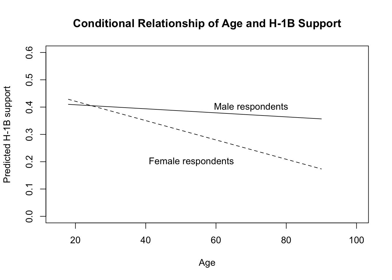
Considering the results, we can conclude that the relationship between H-1B support and age is indeed conditional on sex. Female respondents are on average more opposed to H-1B visas, but the link between age and H-1B support is weaker among male respondents than female respondents (which is indicated by a less steep regression slope). As a result, according to the model with interaction effects, we see sex differences in immigration support among older, but less among younger respondents. Or another way of thinking about this is the relationship between age and H1-B visa support depends on sex.