2 Measurement Theory and Error
Topics: Definition of measurement error. What does it mean for measurements to be fair or unfair? Measurements as functions of indicators. Consequences of measurement error for subsequent analyses.
Required reading:
- Chapters 3, 4 & 5, Pragmatic Social Measurement
Further reading:
Applications - Political Science
- Asher, Herbert B. “Some consequences of measurement error in survey data.” American Journal of Political Science (1974): 469-485.
- Achen, Christopher H. “Proxy variables and incorrect signs on regression coefficients.” Political Methodology (1985): 299-316.
- Bartels, Larry M. “Messages received: The political impact of media exposure.” American political science review 87.2 (1993): 267-285.
Applications - Health
- Butler, Joseph S., et al. “Measurement error in self-reported health variables.” The Review of Economics and Statistics (1987): 644-650.
- Alan B. Krueger and David A. Schkade. “The Reliability of Subjective Well-Being Measures” Journal of Public Economics 2008 Aug; 92(8-9): 1833–1845.
Further Theory
2.1 Seminar
You can also directly load the data file into R from the web with the following command:
region_data <- read.csv(url("https://uclspp.github.io/POLS0013/4_data/week-2-region.csv"))
constituency_data <- read.csv(url("https://uclspp.github.io/POLS0013/4_data/week-2-constituency.csv"))
In this assignment, we are going to use a combination of real data and simulations in order to try to better understand the consequences of measurement error in an explanatory variable. We are also going to create a new measure for the first time, albeit not a very good one.
The core measurement problem of the assignment is trying to measure the results of the 2016 referendum on EU membership in the UK at the level of UK parliamentary constituencies. This is a measurement problem because the UK used different electoral geography for reporting the results of the 2016 referendum than the parliamentary constituencies used in the 2015 and 2017 general elections. The 2016 referendum was reported at the level of local authorities, of which there are 380 in England, Scotland and Wales. That same area includes 632 parliamentary constituencies, each of which sends one MP to Parliament. For a number of applications, it is useful to have a measure of how the voters in a constituency voted in the referendum, but there is no official answer, we have to come up with a measurement strategy.
The best available measures were developed by Hanretty (2017), and are much more accurate than anything we can do easily here because they use details of the geographic/demographic overlap between the different boundaries to aid in imputation. We will treat these as if they are the right answer, even though they are not exactly the right answer.
We are going to use a very simple measurement strategy to develop our own measures. Both local authorities and parliamentary constituencies are nested within the larger geography of (NUTS 1) UK regions, of which there are 11 in England (9), Scotland (1), and Wales (1). Here is the measurement strategy we are going to follow:
- Fit a regression model predicting 2016 leave share using 2015 general election vote for the UK Independence Party at the region level. This is a regression with eleven data points and one explanatory variables.1
- Construct fitted values from the regression model for all 632 constituencies in England, Scotland and Wales using the 2015 general election vote in that constituency.
This is an example of a measurement strategy that is based on calibrating the relationship between a set of indicators (vote in the 2015 election) and the target of the measurement (vote in the 2016 referendum) and then extrapolating to a new set of units. This provides a way of measuring what we want to measure because whereas the 2016 referendum vote is not available on the geographic boundaries that we are interested in (parliamentary constituencies), the 2015 election vote was available on those geographic boundaries. Because both votes are available at the region level, we can use that level of geography to “translate” between the two. How well this works depends on how strong the relationship is between the indicators and the target of the measurement, and whether that relationship is similar in the units on which we train or calibrate the model (regions) to the relationship in the units on which we apply that model to construct fitted values.
- Load the region data file
chapter-2-region.csvand plot the variableLeave16(y) as a function ofUKIP15(x).
library(ggplot2)
library(ggthemes)

p <- ggplot(region_data, aes(x=UKIP15, y=Leave16,col=Region)) +
  geom_point(size=2) +
  geom_text(aes(label=Region), hjust = 0, nudge_x = 0.5,size=3) +
  scale_x_continuous("UKIP Vote 2015",limits = c(0,25)) +
  ylab("Leave Vote 2016") +
  theme_bw() +
  theme(legend.position = "none")
p
- Fit a simple linear regression predicting
Leave16usingUKIP15. Interpret the coefficient onUKIP15. What do we learn from the \(R^2\) of the model? Add a regression line to your plot from Q1.
##
## Call:
## lm(formula = Leave16 ~ UKIP15, data = region_data)
##
## Residuals:
##     Min      1Q  Median      3Q     Max
## -4.8052 -0.6415  0.1746  1.6080  2.9430
##
## Coefficients:
##             Estimate Std. Error t value Pr(>|t|)
## (Intercept)  32.6402     2.4478  13.335 3.12e-07 ***
## UKIP15        1.5105     0.1758   8.592 1.25e-05 ***
## ---
## Signif. codes:  0 '***' 0.001 '**' 0.01 '*' 0.05 '.' 0.1 ' ' 1
##
## Residual standard error: 2.519 on 9 degrees of freedom
## Multiple R-squared:  0.8913, Adjusted R-squared:  0.8793
## F-statistic: 73.83 on 1 and 9 DF,  p-value: 1.246e-05
The coefficient on UKIP15 tells us about the linear association between UKIP15 and Leave16. For each additional percent of vote share that UKIP received in 2015 in a region, leave received, on average, an additional 1.51 percentage point vote share in 2016 in that region (according to our linear model).

The model fits pretty well by the standards of \(R^2\), with 89% of the variation across the 11 regions in 2016 leave vote share explained/predicted by 2015 UKIP vote share.
- Load the constituency level data file
chapter-2-constituency.csvand construct fitted values for each constituency using the variableUKIP15from that file plus the fitted model. You can either do this by manually constructing the fitted values using the estimated coefficients for the intercept andUKIP15or using apredict()command with thenewdataargument set to the constituency dataframe.
- Plot the fitted values you constructed in Q3 against Chris Hanretty’s estimates (the variable
Leave16_Hanrettyfromchapter-2-constituency.csv). Add a line to the plot with intercept 0 and slope 1. What does this line correspond to? What do the deviations of the points from the line correspond to?
p2 <- ggplot(constituency_data,aes(x=Leave16_Hanretty,y=Leave16_UKIP15)) +
  geom_point(size=2,col="darkgray") +
  geom_abline(intercept = 0, slope = 1,col="red",size=1) +
  xlim(0,100)+ ylim(0,100) +
  xlab("Leave 2016 - Hanretty Estimates") + ylab("Leave 2016 - UKIP15 Estimates") +
  theme_bw()

p2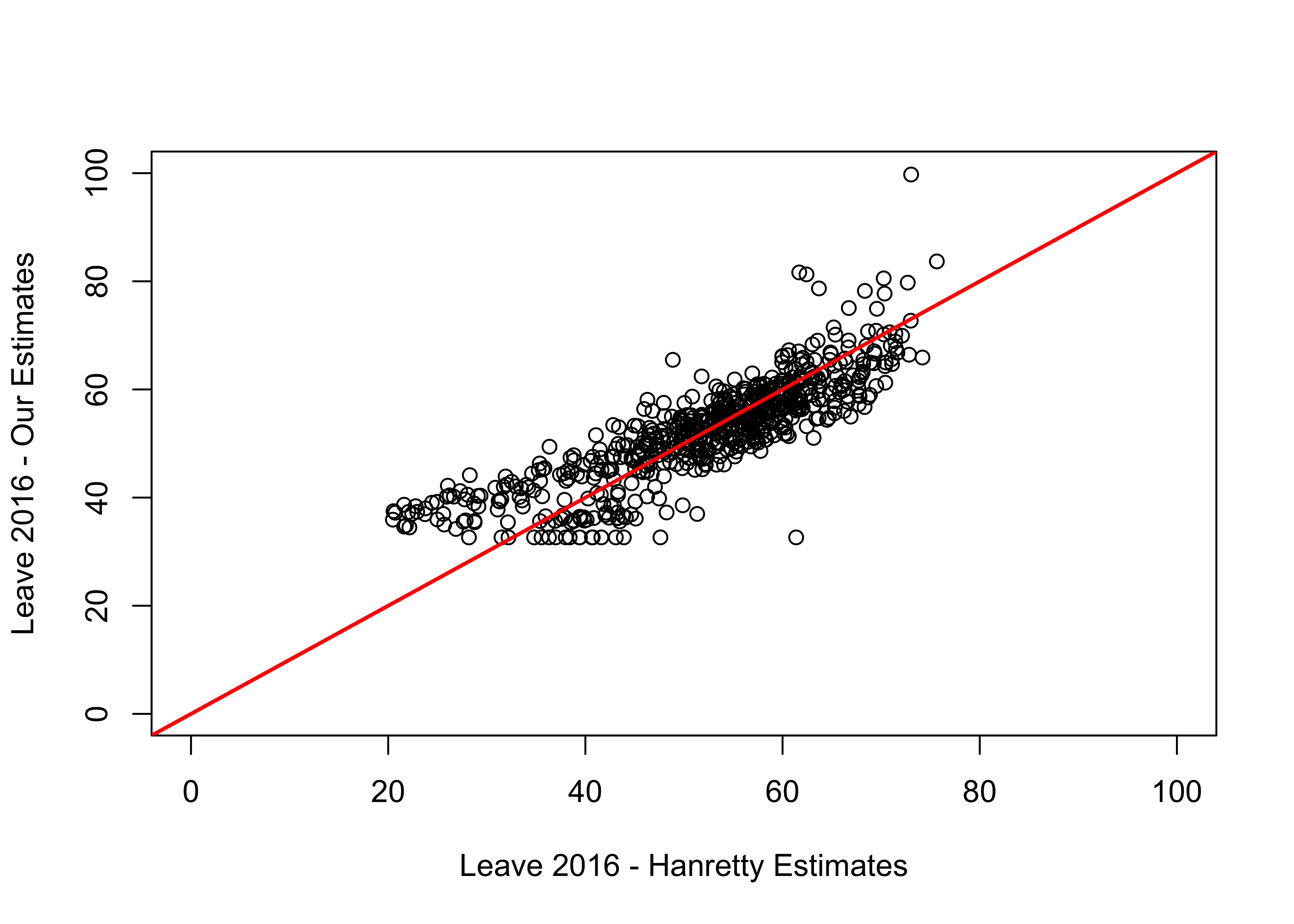
The line with intercept 0 and slope 1 corresponds to the points where the x and y variables are equal, which is to say that our estimates exactly match the Hanretty estimates. Since we are assuming that the Hanretty estimates are much more accurate than ours, the deviations from the line are errors in our measure.
- Why is there a horizontal row of data points at the bottom of the plot? Hint: Compare the value of these points to the coefficients from the regression model we used to form our measure.
Those points correspond to constituencies where UKIP had no candidate and therefore received a vote share of 0. The fitted values are therefore equal to the intercept of the regression model. The relationship between UKIP vote and Leave vote is obviously not going to be the same in places where UKIP had no candidate and where they did have a candidate. This is a limitation of this measurement strategy.
- What are the mean and standard deviation of our measurement errors (if Chris Hanretty’s estimates are correct)? What is the correlation between the measurement error and the Hanretty estimates?
# Mean of measurement error = Bias
mean(constituency_data$Leave16_UKIP15 - constituency_data$Leave16_Hanretty)
## [1] 0.375503# SD of measurement error = Variance
sd(constituency_data$Leave16_UKIP15 - constituency_data$Leave16_Hanretty)## [1] 6.075926# Corelation of measurement error with mu = Miscalibration
cor(constituency_data$Leave16_UKIP15 - constituency_data$Leave16_Hanretty, constituency_data$Leave16_Hanretty)## [1] -0.5188962The measurement error is the difference between our estimates and Hanretty’s estimates (since we assume that the latter are the correct ones). The mean of the measurement error tells us about the bias of the measure, i.e. by how much our measure is wrong, on average - in this case 0.38 percentage points which seems okay.
The standard deviation tells us about the variance of the measure, i.e. by how much more wrong than the mean error our measure is, on average - in this case about 6 percentage points, which is arguably not great.
There is also some evidence of miscalibration as the correlation between the measurement error and Hanretty’s estimates is -0.52. The negative correlation means that the measurement error (difference between our and Hanretty’s estimates) is larger where Hanretty’s estimates are lower. In other words, our measure appears to have more measurement error at lower values of the target concept (Leave vote). This can also be seen in the polot from question 4, where we see that there is more spread from the line for constituencies with a smaller Leave share.
- How much of \(\mu\) is in \(m\)? Calculate and report the correlation, \(R^2\) as well as Kendall’s \(\tau\) between our measure and Hanretty’s estimates.
## [1] 0.8472791## [1] 0.7178818## is the same as
summary(lm(constituency_data$Leave16_UKIP15~constituency_data$Leave16_Hanretty))$r.squared## [1] 0.7178818# Kendall's tau
cor(constituency_data$Leave16_UKIP15,constituency_data$Leave16_Hanretty, method = "kendall")## [1] 0.6929853The (Pearson) correlation coefficient between the two measures is 0.85, quite a strong correlation by most standards. Looking at the \(R^2\), we see that 72% of the variation in our measure is co-variation with Hanretty’s estimates (our \(\mu\) in this case). Finally, by looking at Kendall’s \(\tau\), we see that about 70% of pairwise comparisons between the two measures are ordered in the same direction.
Combining the information gained from this and the previous question, we can conclude that, even though the measures correlate quite strongly with a correlation coefficient of about 0.85, there is clearly a substantively significant amount of measurement error, i.e. mismatch between our measure and Hanretty’s.
- Another measurement strategy that we could have followed would be to simply assume that all constituencies in each region had the same Leave vote share as the region overall. One way to do this is with the following command (change the
dataandnewdataarguments to match how you have saved your datasets).
Evaluate whether this
Region-based measure is a better or worse measure of Leave vote share in constituencies than theUKIP15-based measure we constructed previously, by comparison to Chris Hanretty’s estimates. To do this, you will need to repeat some of the above analyses that we did for theUKIP15-based measure and then make a judgment call based on what you find.
constituency_data$Leave16_Region <- predict(lm(Leave16~Region,
                                               data=region_data),
                                            newdata = constituency_data)

# ggplot
p3 <- ggplot(constituency_data,aes(x=Leave16_Hanretty,y=Leave16_Region)) +
  geom_point(size=2,col="darkgray") +
  geom_abline(intercept = 0, slope = 1,col="red",size=1) +
  xlim(0,100)+ ylim(0,100) +
  xlab("Leave 2016 - Hanretty Estimates") + ylab("Leave 2016 - Region Estimates") +
  theme_bw()

library(patchwork)
p2 + p3 + plot_layout(nrow=1)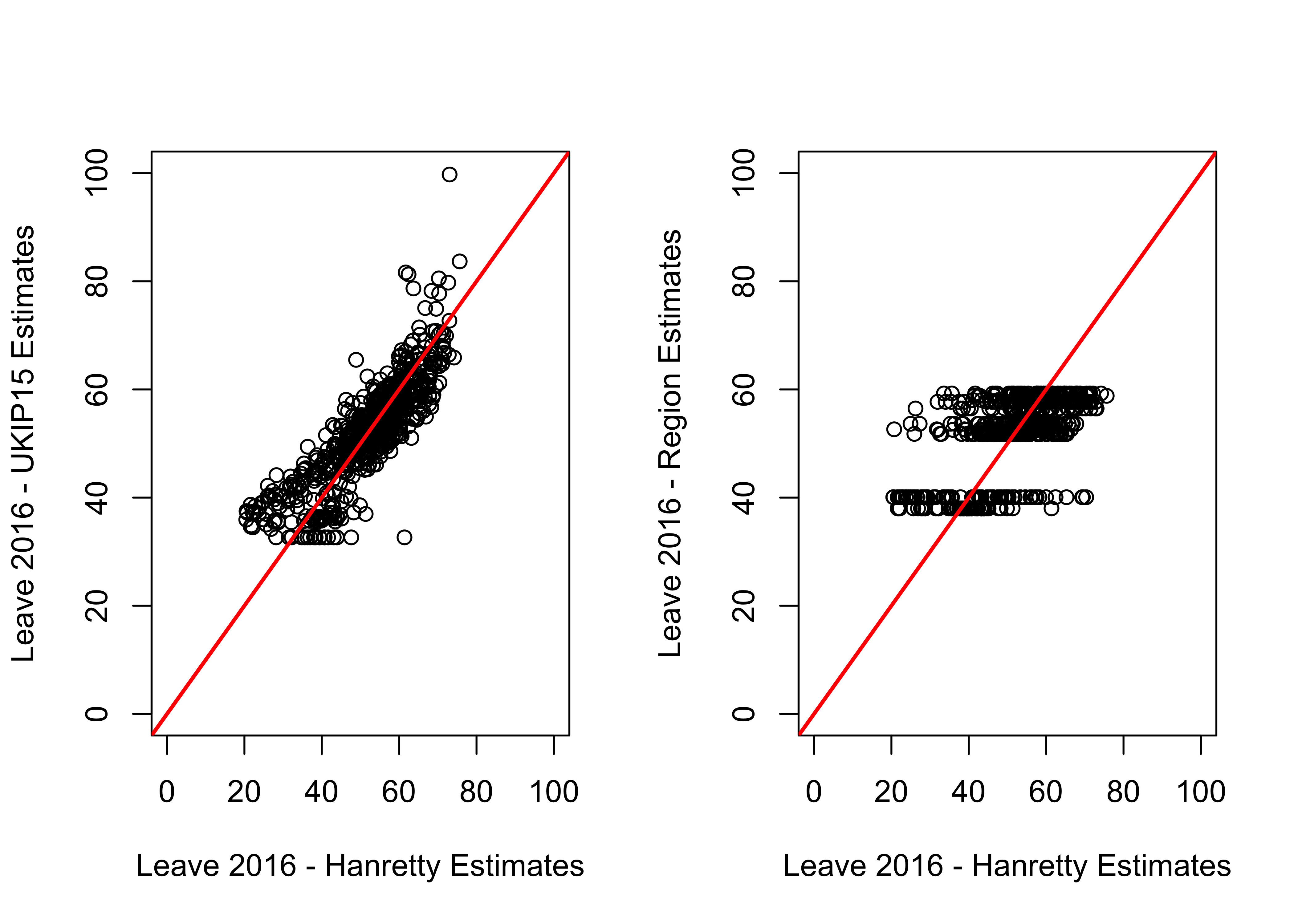
## [1] -0.1379747## [1] 9.016775## [1] 0.6152754The standard deviation of the Region-based measure’s errors with respect to the Hanretty measures are substantially worse than that of the UKIP15-based measure’s errors - it is more wrong than the mean error by about 9 percentage points on average. The correlation is substantially lower as well. It looks like the UKIP15-based measure is probably better than the Region-based measure.
- Now imagine we want to study patterns in the Conservative Party’s gains between the 2015 and 2017 elections. We have a theory that the Conservative Party will have gained more votes in places that supported Leave in the referendum to a greater extent. We want to assess how strong that relationship is. Estimate three regression models for the change in Conservative vote share between 2015 and 2017, one using our
UKIP15-based estimates of the Leave vote on constituency boundaries, one using ourRegion-based estimates, and one using the Hanretty estimates. You will need to construct the variable for the Conservative vote share change fromCon15andCon17in the constituency data.
constituency_data$ConGain1517 <- constituency_data$Con17 - constituency_data$Con15
lm_hanretty <- lm(ConGain1517~Leave16_Hanretty,data=constituency_data)
lm_ukip15 <- lm(ConGain1517~Leave16_UKIP15,data=constituency_data)
lm_region <- lm(ConGain1517~Leave16_Region,data=constituency_data)

# For a quick look at the models in the console, you can use the command screenreg
# from the texreg package. To do this, uncomment the following lines.
# install.packages("texreg")
# texreg::screenreg(list(lm_hanretty,lm_ukip15,lm_region))
# For a slightly more formatted output in either word format or Rmarkdown, you can use modelsummary
# it has a lot of things you can customise, although finding our what to do takes a bit of time and
# a *lot* of searching/trial and error. But if you want nice regression tables, which may be useful
# in your dissertation too, it might be time worth investing.
# But please remember that any extra formatting and new functions used for that are not part of the
# main learning outcomes of the module, it's all just in case you need/want it!
library(modelsummary)
library(tidyverse)
modelsummary(list(lm_hanretty,lm_ukip15, lm_region),
stars = T,
fmt = 2,
coef_rename = function(x) {
x <- str_replace(str_c(x,")"), "Leave16_", "Leave vote share (")
str_replace(x, ".Intercept.*", "Intercept")},
gof_map = c("nobs","r.squared","adj.r.squared"))| (1) | (2) | (3) | |
|---|---|---|---|
| Intercept | -7.18*** | -5.99*** | 1.35 |
| (1.05) | (1.29) | (1.87) | |
| Leave vote share (Hanretty) | 0.25*** | ||
| (0.02) | |||
| Leave vote share (UKIP15) | 0.23*** | ||
| (0.02) | |||
| Leave vote share (Region) | 0.09* | ||
| (0.04) | |||
| Num.Obs. | 632 | 632 | 632 |
| R2 | 0.208 | 0.124 | 0.010 |
| R2 Adj. | 0.206 | 0.122 | 0.008 |
| + p < 0.1, * p < 0.05, ** p < 0.01, *** p < 0.001 | |||
All three models recover positive and significant coefficients on the Leave share variable. There is clear evidence that the Conservatives gained more between 2015 and 2017 in seats where the Leave vote was higher. However the magnitude of this relationship is somewhat smaller using our UKIP15-based measure and very substantially smaller using the Region-based measure.
- Given the material in the lecture, what are some possible explanations for these differences in the coefficients from Q8 (again, maintaining the assumption that the Hanretty estimates are actually correct)?
One possible explanation for why we see these patterns is attenuation bias due to having measurement error in the explanatory variables in the model (Attenuation bias refers to when the regression line is biased towards zero (i.e. flatter) because of error in the independent variable(s)). We already saw in Q7 that the Region-based measure had greater measurement error than the UKIP15-based measure, which is consistent with the idea that there is greater attenuation bias, and therefore a smaller coefficient, when we use the Region-based measure than when we use the UKIP15-based measure.
This is likely not the entire explanation though, because the measurement error was not that much bigger (standard deviation of 9 vs 6), and the coefficient for predicting Conservative gains is far smaller (0.09 vs 0.23).
The other possible explanation is one that involves measurement error in the explanatory variable that is correlated with the outcome measure. This is harder to reason through, but it is probably at least part of the problem. The measurement errors in the UKIP15-based and Region-based measures are correlated with the change in Conservative vote share from 2015 to 2017, meaning that the measurement error in the independent variable is not the same at different values of the dependent variable:
cor(constituency_data$Leave16_UKIP15 - constituency_data$Leave16_Hanretty,
    constituency_data$ConGain1517)
## [1] -0.2917927cor(constituency_data$Leave16_Region - constituency_data$Leave16_Hanretty,
constituency_data$ConGain1517)## [1] -0.500479Both correlations are negative, meaning that, at high values of ConGain1517, measurement error is relatively lower (although note this could mean negative measurement error, and not necessarily less measurement error). These negative correlations between errors \(\epsilon_x\) in \(x\) and the value of \(y\) should yield a negative bias in the \(\beta\) coefficient. This bias will be in the same direction as the attenuation bias, and will again be worse for the Region-based measure than the UKIP15-based measure. It may be better to look at this graphically.
library(ggthemes)
library(wesanderson) # This has colors based on wes anderson's movies! What??!

ggplot(constituency_data,aes(x=ConGain1517)) +
  geom_hline(yintercept = 0, size=1) +
  geom_point(aes(y=Leave16_UKIP15-Leave16_Hanretty,col ='UKIP15 Measure'), size=1,alpha=.5) +
  geom_smooth(aes(y=Leave16_UKIP15-Leave16_Hanretty,col ='UKIP15 Measure'),method = "lm") +
  geom_point(aes(y=Leave16_Region-Leave16_Hanretty,col ='Region Measure'), size=1,alpha=.5) +
  geom_smooth(aes(y=Leave16_Region-Leave16_Hanretty,col ='Region Measure'),method = "lm") +
  ylab("Measurement Error") + xlab("Conservative Gain 15-17") +
  scale_color_manual("",values = c('UKIP15 Measure' = wes_palette("FantasticFox1")[3],
                                'Region Measure' = wes_palette("FantasticFox1")[5])) +
  theme_clean() +
  theme(plot.background = element_rect(color = NA),
        legend.position = "bottom")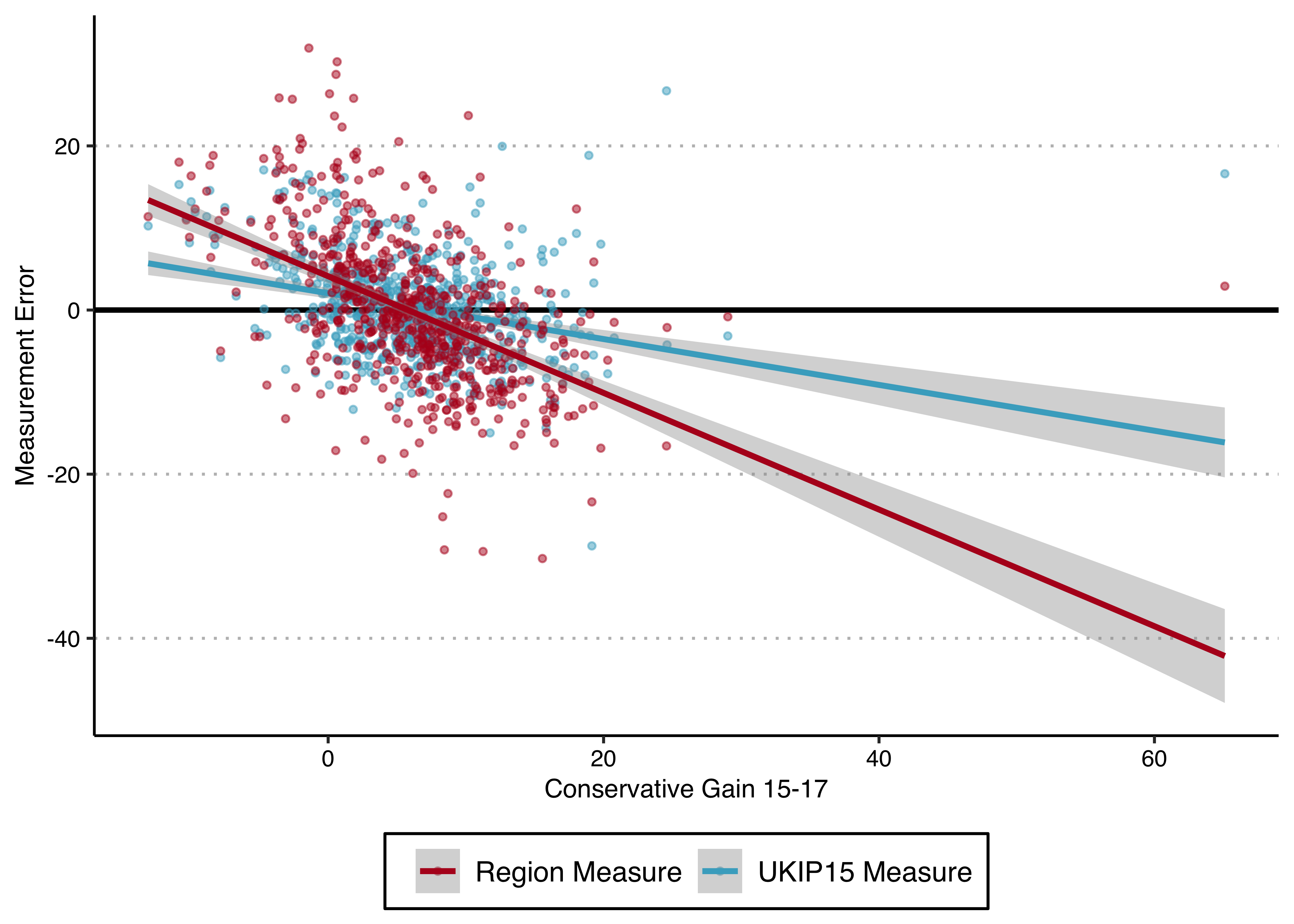
This figure shows us that both measures tend to over-estimate the Leave vote in constituencies where the Conservatives made less (or no, or negative) gains, and under-estimate it in constituencies where the Conservatives made large gains. And this is even more pronounced for the Region measure than the UKIP2015 measure. (More or less) intuitively therefore, if the x variable is less high (low) than it should be for a high (low) values of y, the regression line will be less steep, i.e. the regression coefficient smaller, than it should be.
2.2 Quiz
- Which of the following does not apply to measurement error?
- It is the difference between a measure \(m\) and the target concept \(\mu\)
- A measure can be wrong by being biased (the expected value (mean) of the measurement error is not 0)
- We always know what the measurement error is
- A measure can be wrong by varying to much (the variance of the measurement error is larger than 0)
- A measure can be wrong by being miscalibrated (the correlation between measurement error and target concept is not 0)
- Which of the following refers to whether a measure captures the right thing?
- Precision
- Reliability
- Variance
- Bias
- What does Kendall’s \(\tau\) measure?
- The proportion of pairwise comparisons between points that are ordered in the same direction
- The proportion of overall variance that is explained by the covariance of X and Y (or \(m\) and \(\mu\) if talking about a measure)
- The correlation between a measure \(m\) and the target concept \(\mu\)
- The difference between the expected and observed frequencies in a contingency table
- What does separation mean, in the context of measurement?
- That, given the same value in the target concept, the measurements should be the same.
- That, given the same value in the measurement, the true value should not be systematically different at different values of X.
- That, given the same value in the target concept, the measurements should not be systematically different at different values of X.
- That knowing X about an individual \(i\) should not convey any further information about the likely value \(\mu_i\), once we know \(m_i\).
- Why can separation and sufficiency of a measure m not be jointly satisfied, if the target concept mu does indeed vary by X?
- Because improving validity always comes to some extent at the expense of reliability and vice-versa.
- Because if both the distribution of mu conditional on m and the distribution of m conditional on mu are independent of X, then the unconditional joint distribution of m and mu cannot be dependent on X. In other words, the target concept mu cannot vary by X.
- Because it is more important to improve separation than sufficiency.
- It is actually possible to satisfy both, since measurement error is always constant across values of X
- Which of the following does not have consequences for subsequent analyses?
- Measurement error in the dependent variable
- Measurement error in the control/conditioning variables
- Measurement error in the unobservable confounders
- Measurement error in the independent variable
References
As I said, this is not a very good measurement strategy, although it isn’t terrible either. If we had more data points, we might include more explanatory variables (indicators) such as vote for the Conservative Party, etc.↩︎