9 Unsupervised Scale Measurement II: Categorical Indicators
Topics: Item response theory for data with binary and/or ordinal indicators.
Required reading:
- Chapter 12, Pragmatic Social Measurement
Further reading:
Theory
- Bartholomew et al. (2008), Ch 8 & 9
Applications
- Shawn Treier and Simon Jackman, “Democracy as a Latent Variable” American Journal of Political Science. Volume 52, Issue 1. January 2008. Pages 201-217
- Shawn Treier, D. Sunshine Hillygus, “The Nature of Political Ideology in the Contemporary Electorate”, Public Opinion Quarterly, Volume 73, Issue 4, Winter 2009, Pages 679–703
- Treier, S. (2010). Where Does the President Stand? Measuring Presidential Ideology. Political Analysis, 18(1), 124-136.
9.1 Seminar
The data for this assignment are an extract from the 2017 British Election Study, conducted using face to face interviews.We are going to consider strategies for analysing these data, both based on tallying up correct and incorrect answers, and also based on using IRT models.
There are a number of questions we might use on this survey that are suitable for analysis with IRT, and the data extract includes a couple of extra sets that you can use if you are interested. The one that we will focus on is the “battery” of questions on political knowledge. These are six items, on which respondents could give True, False, or “Don’t Know” responses:
- (
x01_1) Polling stations close at 10.00pm on election day. - (
x01_2) No-one may stand for parliament unless they pay a deposit. - (
x01_3) Only taxpayers are allowed to vote in a general election. - (
x01_4) The Liberal Democrats favour a system of proportional representation for Westminster elections. - (
x01_5) MPs from different parties are on parliamentary committees. - (
x01_6) The number of members of parliament is about 100.
The correct answers to these six items are True, True, False, True, True, and False, respectively.
Use the following code to tidy up these six items, and re-order the factor levels to run c("False","Don't Know","True"). Note that these are not R logical values TRUE and FALSE, these are the character strings of the responses given to the survey.
knowledge_battery <- bes[,c("x01_1","x01_2","x01_3","x01_4","x01_5","x01_6")]
for (k in 1:ncol(knowledge_battery)) {
  knowledge_battery[,k] <- replace(knowledge_battery[,k],knowledge_battery[,k] == "Not stated","Don't know") # there are few of these, but easier to treat them as don't know
  knowledge_battery[,k] <- droplevels(knowledge_battery[,k])
  knowledge_battery[,k] <- relevel(knowledge_battery[,k],"False")
}
You can quickly see the distribution of responses using the following command:
| x01_1 | x01_2 | x01_3 | x01_4 | x01_5 | x01_6 | |
|---|---|---|---|---|---|---|
| False | 91 | 489 | 1932 | 175 | 120 | 1528 |
| Don’t know | 184 | 596 | 115 | 931 | 690 | 457 |
| True | 1919 | 1109 | 147 | 1088 | 1384 | 209 |
For this assignment, you will also need to install and load the R library ltm:
install.packages("ltm")
library(ltm)

# you may also need these packages
library(kableExtra)
library(magrittr)
library(ggplot2)
library(ggthemes)
- Use the object
knowledge_batteryto create a new objectbinary_correctwhich is 1 for responses that are correct, and 0 for responses that are don’t know or which are incorrect. The object you create should have the same dimensions and column/row order asknowledge_battery. Create a histogram of the number of total correct answers by respondent.
# There are many ways to do this recoding.

# the 'manual' (less exciting) way
binary_correct <- knowledge_battery

binary_correct$x01_1 <- ifelse(binary_correct$x01_1=="True",1,0)
binary_correct$x01_2 <- ifelse(binary_correct$x01_2=="True",1,0)
binary_correct$x01_3 <- ifelse(binary_correct$x01_3=="False",1,0)
binary_correct$x01_4 <- ifelse(binary_correct$x01_4=="True",1,0)
binary_correct$x01_5 <- ifelse(binary_correct$x01_5=="True",1,0)
binary_correct$x01_6 <- ifelse(binary_correct$x01_6=="False",1,0)

# the slightly more exciting and arguably neater way (with tidyverse)
library(tidyverse)
correct_answers <- c("True","True","False","True","True","False")
binary_correct <- knowledge_battery |>
  mutate(across(which(correct_answers == "True"), ~ ifelse(.=="True",1,0)),
         across(which(correct_answers == "False"), ~ ifelse(.=="False",1,0)))

# plotting
hist(rowSums(binary_correct),
     xlab="Correct Responses",main="",
     br=seq(-0.5,6.5,1),freq=FALSE)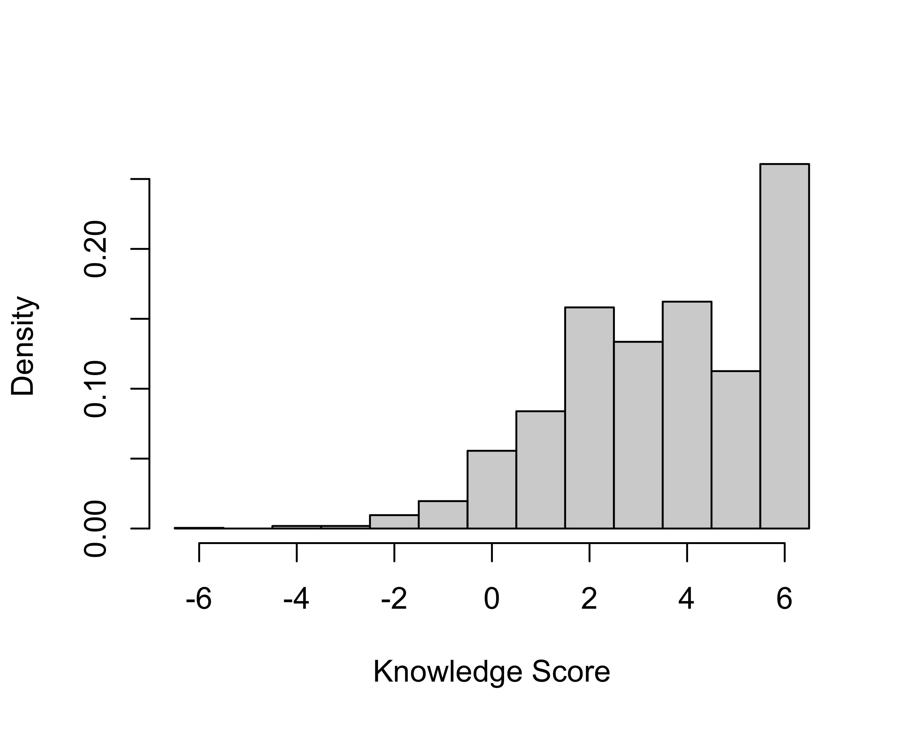
- Use the object
knowledge_batteryto create a new objectternary_correctwhich is 1 for responses that are correct, 0 for responses that are don’t know, and -1 for responses which are incorrect. The object you create should have the same dimensions and column/row order asknowledge_battery. Create a histogram of the total number of “points” for each respondent, where each incorrect response counts as -1, each don’t know response counts as 0, and each correct response counts as 1.
ternary_correct <- knowledge_battery

ternary_correct$x01_1 <- ifelse(ternary_correct$x01_1=="True",1,
                                ifelse(ternary_correct$x01_1=="False",-1,0))
ternary_correct$x01_2 <- ifelse(ternary_correct$x01_2=="True",1,
                                ifelse(ternary_correct$x01_2=="False",-1,0))
ternary_correct$x01_3 <- ifelse(ternary_correct$x01_3=="False",1,
                                ifelse(ternary_correct$x01_3=="True",-1,0))
ternary_correct$x01_4 <- ifelse(ternary_correct$x01_4=="True",1,
                                ifelse(ternary_correct$x01_4=="False",-1,0))
ternary_correct$x01_5 <- ifelse(ternary_correct$x01_5=="True",1,
                                ifelse(ternary_correct$x01_5=="False",-1,0))
ternary_correct$x01_6 <- ifelse(ternary_correct$x01_6=="False",1,
                                ifelse(ternary_correct$x01_6=="True",-1,0))

# version 2 (with tidyverse)
ternary_correct <- knowledge_battery |>
  mutate(across(which(correct_answers == "True"), ~ ifelse(.=="True",1,
                                                           ifelse(.=="False",-1,0))),
         across(which(correct_answers == "False"), ~ ifelse(.=="False",1,
                                                            ifelse(.=="True",-1,0))))

# plotting
hist(rowSums(ternary_correct),
     xlab="Knowledge Score",main="",
     br=seq(-6.5,6.5,1),freq=FALSE)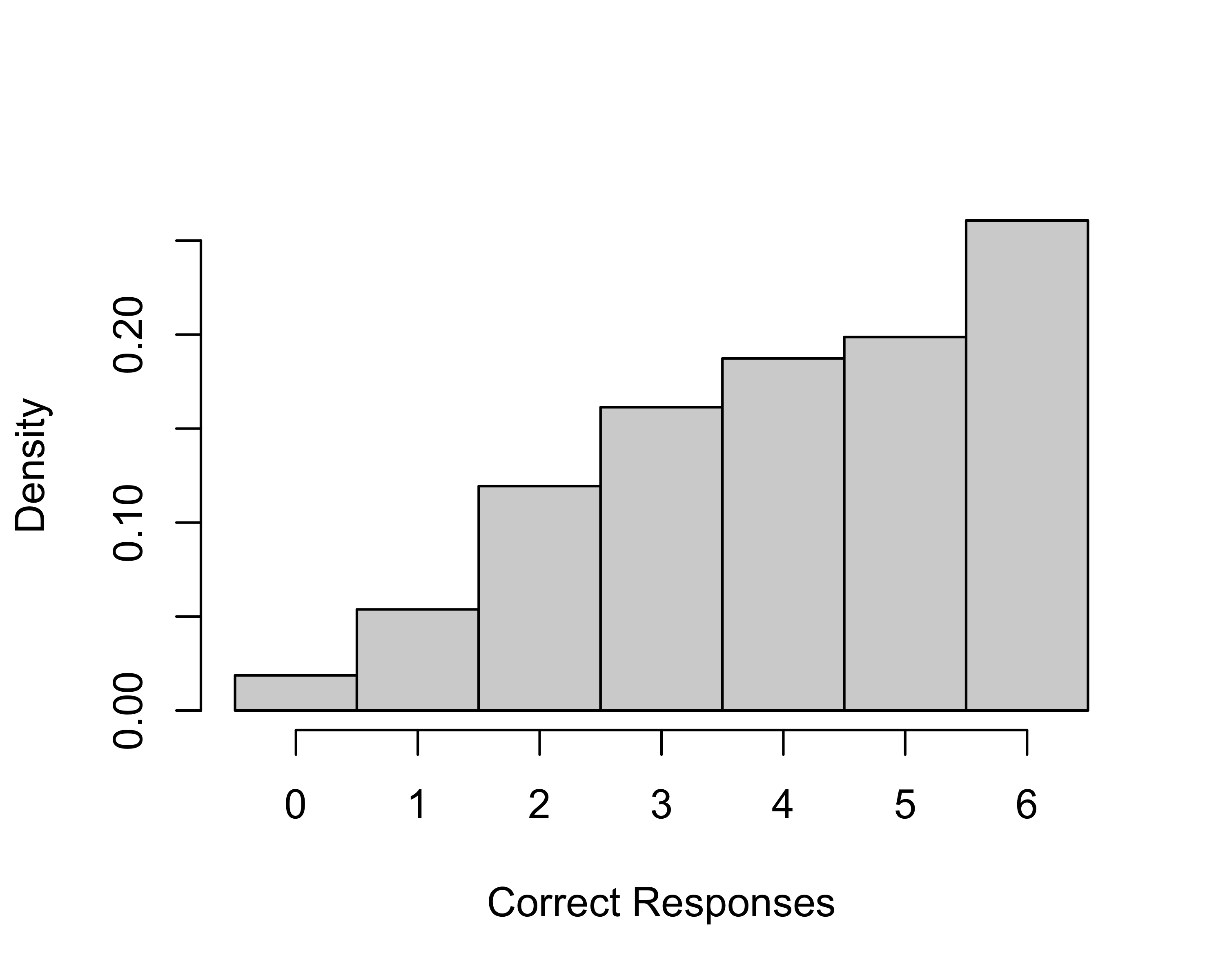
- What potential problem with counting correct answers is addressed by counting incorrect responses as -1 rather than 0 if the goal is to create a measure of political knowledge for respondents to the survey?
Penalizing incorrect answers is a way of correcting for guessing. Someone who knows nothing, but randomly guesses true or false, will get an average of three answers correct and three answer incorrect across six questions. Scoring the incorrect answers as -1 ensures that respondents guessing randomly will get the same score, on average, as those who answer don’t know to all items.
- Use the R function
ltm()to fit a binary IRT model usingbinary_correctas the data (see the code below). Print a summary of the coefficients from the model and use the default plot method for the resulting fitted model object, egplot(ltm_fit), to see the item response/characteristic curves for all six items. Which was the “easiest” knowledge item? Which was the most difficult knowledge item?
##
## Call:
## ltm(formula = binary_correct ~ z1)
##
## Coefficients:
##        Dffclt  Dscrmn
## x01_1  -1.917   1.293
## x01_2  -0.020   1.733
## x01_3  -2.391   0.973
## x01_4   0.011   2.426
## x01_5  -0.460   1.807
## x01_6  -0.761   1.560
##
## Log.Lik: -6698.615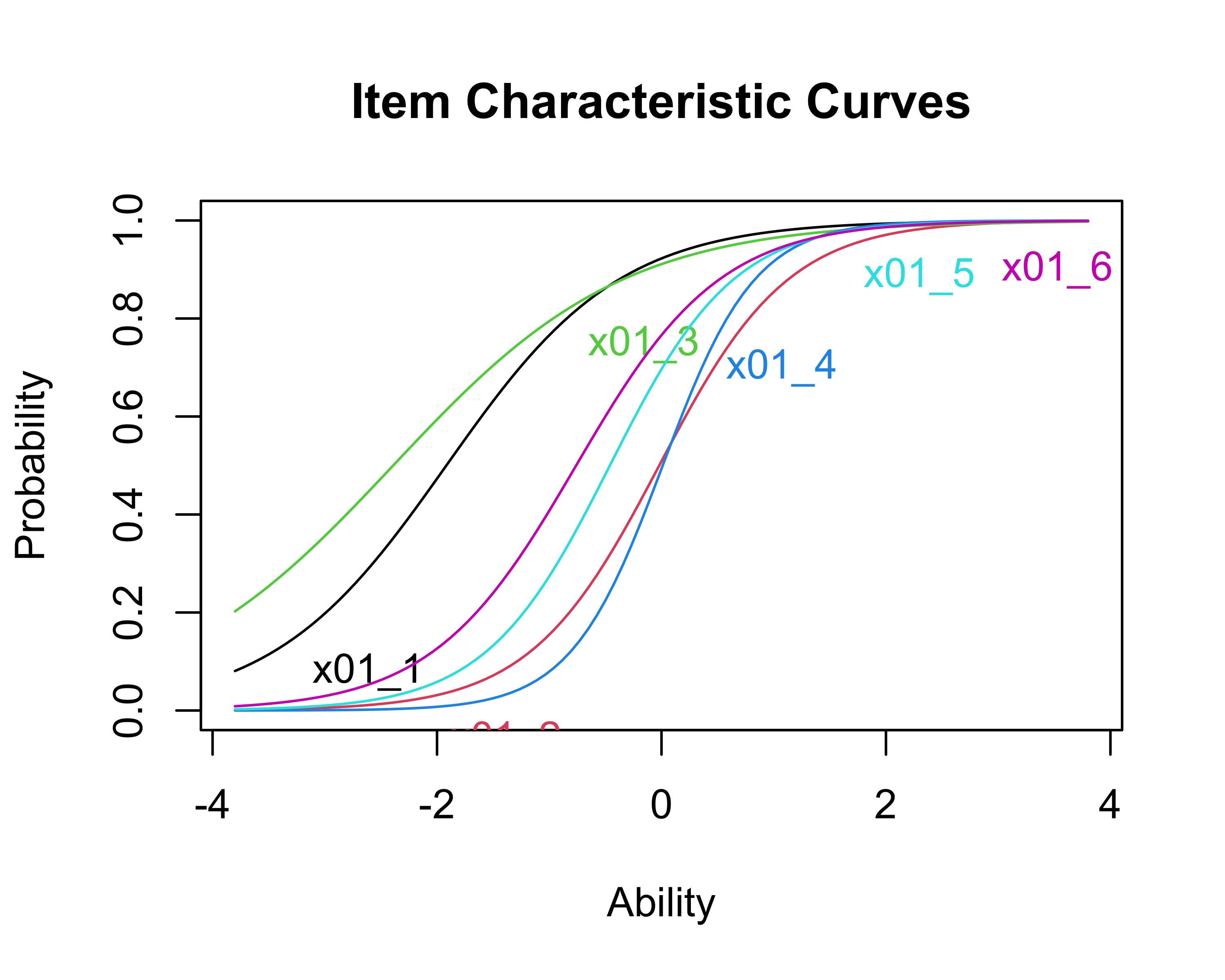
If we examine the coefficients and the plot, we see that item 3 is the easiest item in the sense of having the most negative difficulty parameter, which corresponds to the item which reaches a 0.5 probability of a correct response at the lowest level of the latent variable (labeled ability by default in the R plot). This is the (false) item “Only taxpayers are allowed to vote in a general election.” This is the item that the most respondents answered correctly, 88%.
The most difficult item by difficulty parameter is item 4, although item 2 is very close and has a lower discrimination parameter, which means that individuals at high “ability” are more likely to get item 2 wrong than item 4. Item 4 was correctly answered by 50% of respondents. This is the (true) item “The Liberal Democrats favour a system of proportional representation for Westminster elections.”
- Use the command below to recover the “factor scores” (latent variable estimates) for the binary response IRT model that we just fit. Once you have run this command,
ltm_scores$score.dat$z1will give you the score for each respondent in the original data set. Plot these scores against the number of correct responses per respondent. Explain the pattern that you see and what it tells us about the validity of the two approaches (tallying up correct/incorrect responses vs fitting an IRT model) for measuring political knowledge from these response data. Hint: To get the number of correct responses per respondents you can sum up each row withrowSums(). When plotting, you can usejitter()to create some random noise around the number of correct responses (otherwise everything will overlap and not be very readable).
ltm_scores <- factor.scores.ltm(ltm_fit,resp.patterns=binary_correct)

# put in a data frame for plotting
out <- data.frame(scores = ltm_scores$score.dat$z1,
                  num_correct = rowSums(binary_correct))

# plot
ggplot(out, aes(x=jitter(num_correct),y=scores)) +
  geom_point(size=2,alpha=.5) +
  scale_x_continuous("Correct Responses",breaks = 0:6) +
  scale_y_continuous("Binary IRT Score",breaks = seq(-2,2,0.5)) +
  theme_clean() +
  theme(plot.background = element_rect(color=NA))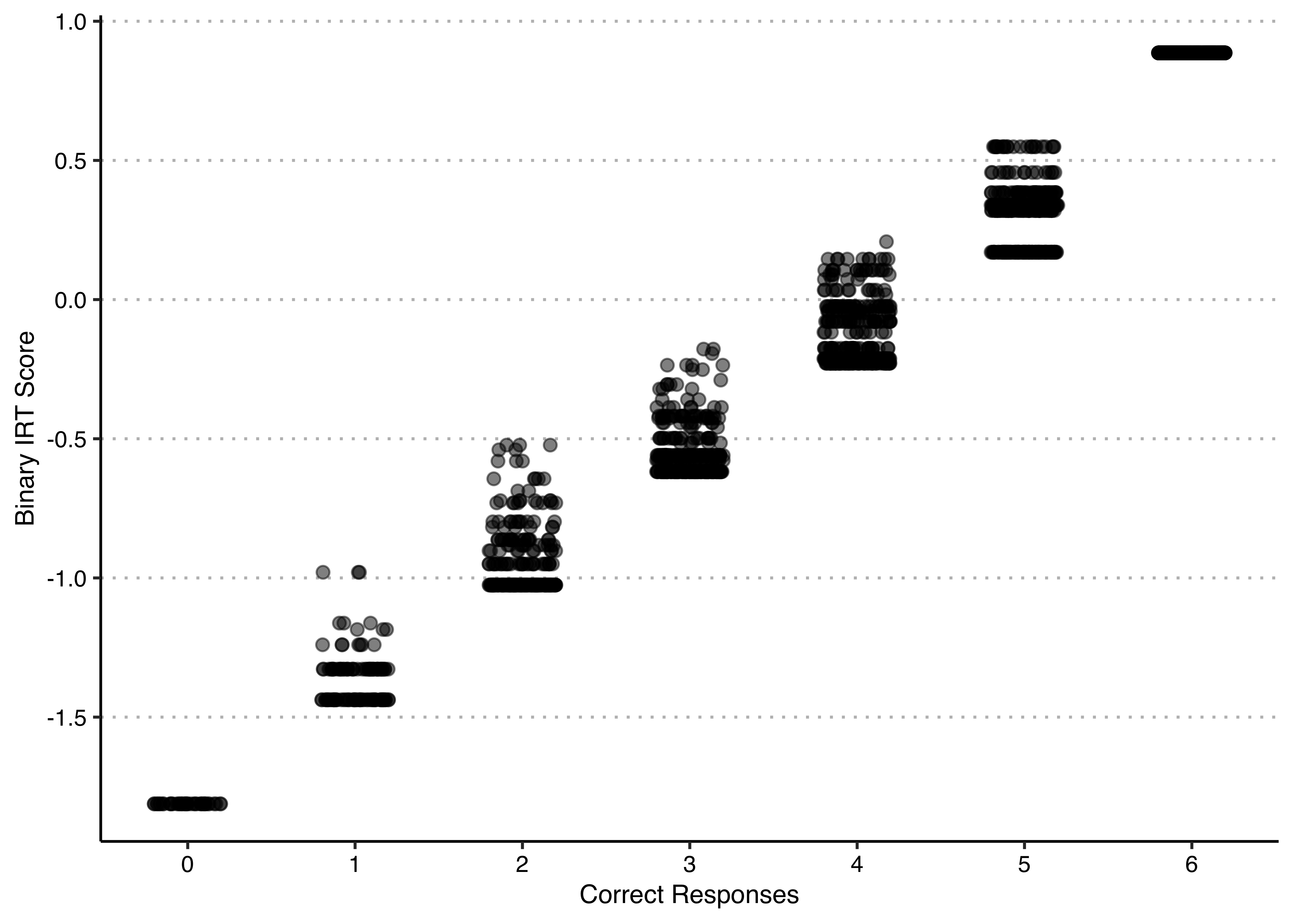
We clearly see that the IRT score is very closely related to the number of correct responses, the correlation between the two measures is 0.99. If you look closely at the plot, you see that, within any given number of correct responses, there are a limited set of possible values of the IRT score. This is because there are only six items in this test, and so there are only a limited number of ways to get a given number of items correct. Because some of the items are easier or more difficult than others, certain patterns of correct and incorrect responses may be more/less frequent than others.
All of these items have positive discrimination parameters, and these are reasonably similar in magnitude, suggesting that this is a reasonable battery of questions for measuring political knowledge and that measures based on tallying up correct/incorrect responses are likely to closely resemble the latent variable from the item response model.
However, this plot may also lead us to question the usefulness of doing a binary IRT model vs simply adding up the correct answers. Essentially, these two seem to agree quite a lot, meaning that there is little that the IRT factor scores tell us that counting the number of right responses doesn’t. But if you didn’t do the IRT model, you would not know that, so I guess it is still useful to at least do it!
- Use the R function
grm()to fit a three-category ordered IRT model usingknowledge_batteryas the data. Print a summary of the coefficients from the model and use the default plot method for the resulting fitted model object, eg.plot(grm_fit), to see the item response/characteristic curves for all six items.
##
## Call:
## grm(data = knowledge_battery)
##
## Coefficients:
##        Extrmt1  Extrmt2  Dscrmn
## x01_1   -2.770   -1.810   1.425
## x01_2   -1.444   -0.085   1.102
## x01_3   -2.412   -3.119  -0.966
## x01_4   -2.031   -0.024   1.674
## x01_5   -2.521   -0.546   1.443
## x01_6   -0.886   -2.206  -1.296
##
## Log.Lik: -9256.759
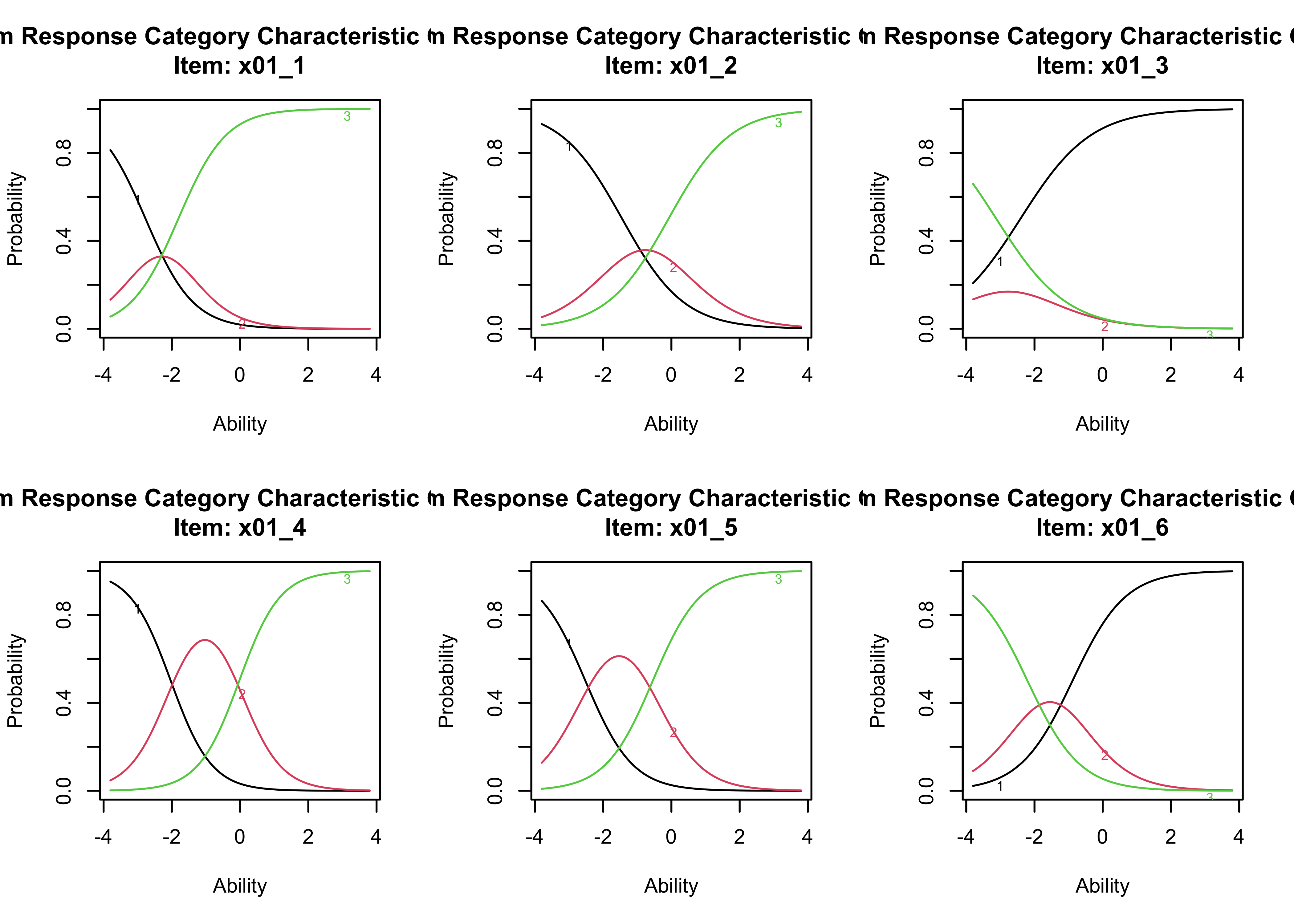
By looking at the coefficients now, we see that there is still one discrimination parameter for each item, but now there are two ‘difficulty’ parameters, because there are two thresholds (from ‘False’ to ‘Don’t know’ and from ‘Don’t know’ to ‘True’). The first one (Extrmt1) tells us the value in the latent factor at which the probabilities of responding ‘False’ vs ‘Don’t know’ or ‘True’ to that particular item are equal. The second one (Extrmt2) tells us the value in the latent factor at which the probabilities of responding ‘False’ or ‘Don’t know’ vs ‘True’ to that particular item are equal. You can think of having two difficulty paramters as, on the one hand, the difficulty of giving a response that indicates lack of knowledge (i.e. ‘don’t know’) vs wrong knowledge and, on the other hand, the the difficulty of giving a response that indicates correct knowledge vs lack of knowledge.
- Examine the signs of the discrimination parameters. What do these tell us about the patterns of responses? What do these tell us about what the latent variable is measuring for each respondent?
A “feature” of factor/IRT models is that they do not assume that all the indicators have the same direction of association with the latent variable, which can be useful when that direction is unknown. One thing we can see in the coefficients and the plots is that two items (3 and 6) have negative discrimination parameters. This is evident in the item response curves because it is the “3” category (the “True” survey response) that becomes most common as ability goes up for items 1, 2, 4 and 5, but it is the “1” category” (the “False” survey response) that becomes most common as ability goes up for items 3 and 6. This is because we have used the original response data rather than recoding it as correct/incorrect. Note that we could have recoded the data as correct/don’t know/incorrect and we would have recovered identical estimates of ability, the only thing that would have changed is that the sign of the parameters would have flipped for the two items that are “reverse” coded (items 3 and 6).
At a more fundamental level, these results tell us that we are measuring something like political knowledge, because being higher on the latent variable is associated with increased probabilities of correct responses on all items.
We can also see clearly in the plots which items received relatively large numbers of “don’t know” responses (items 4 and 5) and which received relatively few (item 3), as this is roughly indicated by the area under the curve showing the probability of giving the “2”/intermediate response.
- Repeat the analysis you did in Q5, but this time for the scores from the ordered IRT model and comparing to
rowSums(ternary_correct)instead ofrowSums(binary_correct). Use the following command to construct the factor scores:
grm_scores <- factor.scores.grm(grm_fit,resp.patterns=knowledge_battery)

out2 <- data.frame(scores2 = grm_scores$score.dat$z1,num_correct = rowSums(ternary_correct))
ggplot(out2, aes(x=jitter(num_correct),y=scores2)) +
  geom_point(size=2,alpha=.5) +
  scale_x_continuous("Correct Responses",breaks = -6:6) +
  scale_y_continuous("Ordered IRT Score",breaks = seq(-3,1,0.5)) +
  theme_clean() +
  theme(plot.background = element_rect(color=NA))
In Q5, we compared IRT scores from the binary model to the number of correct responses, and saw that these were highly correlated. Here, we compare IRT scores from the ordered model (with don’t know as the intermediate category), and see that these are highly correlated with the score based on giving -1 to incorrect responses, 0 to don’t know responses, and 1 to correct responses. These are correlated at 0.91, meaning there is slightly less agreement between the ordinal IRT model and the ternary sum score, suggesting that the IRT model tells us slightly more than just adding up the scores (compared to the binary version).
- Plot the scores from the binary model against those of the ternary model. Discuss what you observe.
results <- data.frame(binary = out$scores, ordered = out2$scores2)

ggplot(results, aes(x=binary,y=ordered)) +
  geom_point(size=2,alpha=.5) +
  scale_x_continuous("Binary IRT Scores (Correct vs Incorrect/Don't Know)",breaks = seq(-2,1,0.5)) +
  scale_y_continuous("Ordered IRT Scores (Incorrect vs Don't Know vs Correct)",breaks = seq(-3,1,0.5)) +
  theme_clean() +
  theme(plot.background = element_rect(color=NA))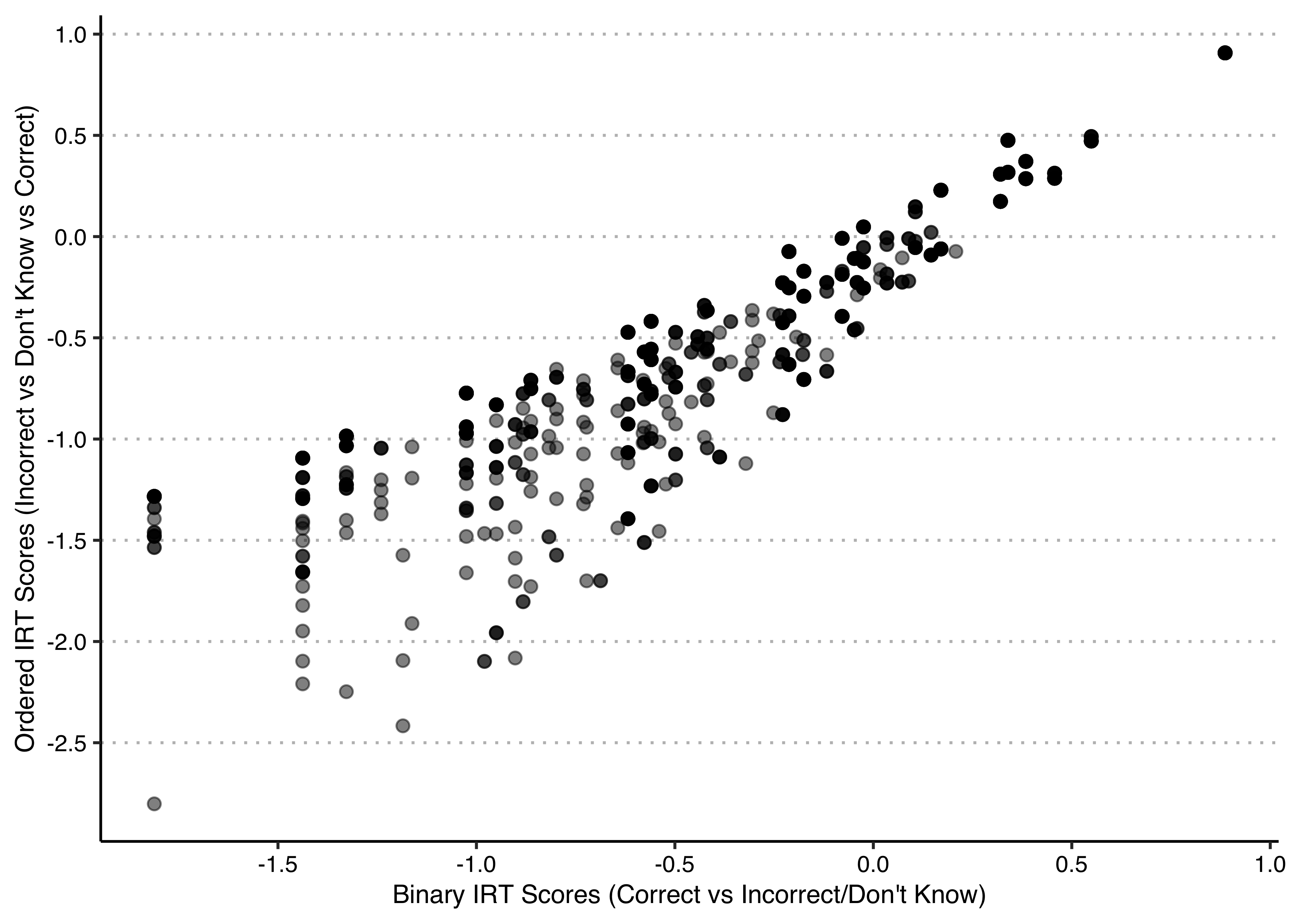
This plot has a distinctive triangular shape. Low scores on the binary IRT score are associated with a range of low to medium scores on the ordered IRT score, but as the binary IRT score increases, the range of associated ordered IRT scores shrinks.
The reason for this is that there are two ways in which you can fail to give the correct answer—you can give the incorrect answer or a don’t know answer—and the two models treat them differently. In the binary model, we treated incorrect answers and don’t know answers as equivalent; in the ordered model, we treated incorrect answers as “worse” than don’t know answers. As a result, at low levels of the scores, where most of the responses are not the correct one, there is potentially a lot of variation in the extent to which respondents gave incorrect answers versus saying they did not know. Those who said don’t know more frequently will score higher under the ordered IRT model than those who gave the incorrect answers more frequently, given the same set of items on which they gave correct answers. The more correct answers (higher binary IRT scores, higher values of x), the less scope there is for this variation in the ordinal IRT scores (values of y) because there are fewer answers that are not the correct one.
- Do you think that it makes sense to treat these response data as ordinal? Does “don’t know” necessarily reflect an intermediate level of knowledge between that of getting the answer wrong and that of getting the answer right?
Treating the don’t know response as intermediate captures the idea that an incorrect response is a more negative signal regarding someone’s political knowledge because it implies that they are likely to have spurious correct responses due to guessing. What the model does not capture is the idea that there might be people who like to guess and that there are other people who do not. There are sources of variation in people’s propensity to give the don’t know response. For example, several studies have found that men are more likely to guess and women are more likely to say they do not know the answer to questions like these (Mondak and Anderson 2004; Lizotte and Sidman 2009; Ferrı́n, Fraile, and Garcı́a-Albacete 2017). Several of these studies note that these differences have the consequence that measuring political knowledge simply by counting correct answers ends up overstating the political knowledge of men relative to women. Greater rates of guessing mean that while men tend to provide more correct answers, they also tend to provide more incorrect answers.
9.2 Quiz
- Which of the following defines Item Response Theory?
- It describes the field of research of public opinion with survey items.
- It describes a class of regression-like models for limited dependent variables.
- It describes a class of factor-analysis like models for limited dependent variables.
- It describes a way of calculating weights with which to aggregate indicators into a measure.
- In a logistic IRT model, what is the linear combination of the coefficients and factors equal to?
- The probability that the response to a given item I is 1.
- The estimated value of the latent factor for a given unit i.
- The log-odds that the latent factor value for a given unit i is 1.
- The log-odds that the response to a given item I is 1.
- Which of the following is not true about the use of the alternative parametrization of a binary logistic IRT model as \(\beta_j(\theta_i-\alpha_j)\)?
- It changes the alpha from a x intercept into a y intercept.
- \(\alpha_j\) can then be interpreted as a ’difficulty’ parameter by representing the minimum value of \(\theta_i\) a unit must have in order for the probability of answering 1 to item I is equal or higher than 50%.
- It only makes sense if most items respond positively to the same latent factor (all/most \(\beta\)’s are positive)
- The procedure to calculate the predicted probabilities of I=1 for a given value of \(\theta\) is the same than with the ‘original’ parametrization.
- How many different regression equations does an IRT model estimate?
- As many as there are units.
- As many as there are items.
- As many as there are factors.
- As many as there are indicator levels.
- Which of the following is incorrect about PCA, EFA and IRT models?
- All will estimate the same number of equations.
- The overall sign of the scale is always arbitrary.
- They are all ways to best summarise the variance in the data.
- They are all ways to measure underlying dimensions that cause the observed data.