7 Supervised Class Measurement
Topics: Assessing whether a target concept should be treated as continuous or categorical. Supervised classification (coding, training).
Required reading:
- Chapter 10, Pragmatic Social Measurement
Further reading:
Theory
- James et al. (2013), Ch 4
- Collier, David, Jody LaPorte, and Jason Seawright. “Putting typologies to work: Concept formation, measurement, and analytic rigor.” Political Research Quarterly 65.1 (2012): 217-232.
Applications
- Anna Luhrmann, Marcus Tannenberg and Staffan I. Lindberg. “Regimes of the World (RoW): Opening New Avenues for the Comparative Study of Political Regimes”
- Rooduijn et al. “The PopuList” A populism classification of European parties from 31 countries.
- Kostas Gemenis. “What to Do (and Not to Do) with the Comparative Manifestos Project Data”
7.1 Seminar
This week, the variables we are going to use are a set of questions about how respondents think about voting. These are four items, on which respondents could give Strong Agree, Agree, Neither Agree nor Disagree, Disagree or Strongly disagree responses:
- (
c02_1) Going to vote is a lot of effort - (
c02_2) I feel a sense of satisfaction when I vote - (
c02_3) It is every citizen’s duty to vote in an election - (
c02_4) Most of my friends and family think that voting is a waste of time.
- Attempt to specify a coding rule for classifying respondents according to whether they “think they have reasons to vote”. That is, we are trying to code respondents into people who think they have reasons to vote and people who do not think they have reasons to vote. You should both write out in words what your coding rule is, and also implement it in
Rcode such that given the values ofc02_1,c02_2,c02_3andc02_4you are able to calculate the classification of each respondent. How many people indicate that they have reason to vote and how many do not, under your coding rule? Note: Your coding rule will involve some judgement calls, and there is no one right answer here (there are nonetheless plenty of wrong answers!). You may decide that not all of the four indicators are relevant to this concept, that is fine. You will need to decide what to do with the small number of respondents who give “Don’t know” responses to one or more of these items, you should aim to classify all respondents.
There are many ways to answer this question. Here is one example of the sort of reasoning that might get you to a coding rule.
The concept we are trying to measure is whether respondents “think they have reasons to vote”. We may decide that only two of these four indicators really reflect “reasons” to vote. For instance, c02_1 “Going to vote is a lot of effort” may not really relevant to the concept, it is more about the costs of voting than the “reasons to” vote. Similarly, while c02_4 “Most of my friends and family think that voting is a waste of time.” could indicate something indirect about social pressure to vote, whether one’s friends and family think that voting is a waste of time is more related to the costs of voting than the reasons to vote. Both of these exclusions are arguable!
Having “reasons to vote” does not mean you need to have all the reasons, so the coding rule is that anyone who says “agree” or “strongly agree” to either c02_2 “I feel a sense of satisfaction when I vote” or c02_3 “It is every citizen’s duty to vote in an election” classifies as having good reasons. Everyone else does not. Thus the R code is:
reason_to_vote <- bes$c02_2 == "Agree" |
  bes$c02_2 == "Strongly agree" |
  bes$c02_3 == "Agree" |
  bes$c02_3 == "Strongly agree"

# this is equivalent to
reason_to_vote <- bes$c02_2 %in% c("Agree","Strongly agree") |
  bes$c02_3 %in% c("Agree","Strongly agree")

table(reason_to_vote)
## reason_to_vote
## FALSE TRUE
## 367 1827## reason_to_vote
## FALSE TRUE
## 0.17 0.8383% of respondents are classified as having a reason to vote. Note that the “Don’t know” responses are being treated as a lack of reason to vote here.
- Cross-tabulate your classification against the variables
turnout_selfandturnout_validated. How well does your classification predict self-reported turnout and validated turnout, respectively?
Note: Validated turnout is not available for all respondents, but involves the British Election Study staff checking the marked voter register after the election to see if the respondent actually voted.
To look at how well our classification predicts self-reported and validated turnout, respectively, we need to look at the latter’s proportions conditioning on values of our classification. Note that this is what we do when running a linear regression: we calculate the average value (in this case proportion) of the dependent variable given particular values of our independent variables.
# self-reported turnout
round(
  prop.table(
    table(
      "turnout_self"=bes$turnout_self,
      reason_to_vote)
    , margin = 2) # 2 to condition on the *second* variable (i.e. reason_to_vote)
  ,3) # 3 digits rounding
## reason_to_vote
## turnout_self FALSE TRUE
## FALSE 0.523 0.148
## TRUE 0.477 0.852## (Intercept) reason_to_voteTRUE
## 0.477 0.375Remember, the intercept is the average self-reported turnout for those for whom our measure said that they did not have a reason to vote (i.e. reason_to_vote=FALSE). Notice that the intercept is equal to the number in the bottom left cell of the table of conditional proportions we calculated above. And, if you add intercept and coefficient, you get the average turnout for those that, according to our measure, had a reason to vote: \(0.477+0.375= 0.852\), which is equal to the bottom right cell of the preceding table.
# validated turnout
round(
  prop.table(table("tunout_validated"=bes$turnout_validated,
                   reason_to_vote),2)
  ,3)
## reason_to_vote
## tunout_validated FALSE TRUE
## FALSE 0.525 0.211
## TRUE 0.475 0.789For self-reported voting, turnout is 85% among those with a reason to vote, and 48% among those without. For validated voting, turnout is 79% among those with a reason to vote, and 48% among those without.
Such a classification of “reasons to vote” does not predict voting all that well overall. It is pretty good at predicting self-reported and validated turnout among those with reasons to vote, according to our measure. However, among those without reasons to vote, our measure is not very good at predicting (no) turnout, since in both cases, 48% still (reported that they) voted.
- Now cross-tabulate your classification against the different combinations of
turnout_selfandturnout_validatedand find out the following:
- the proportion of individuals who said they voted and were recorded as voting have reasons to vote, according to our measure, i.e the true positives.
- the proportion of individuals who said they voted but were not recorded as actually voting have reasons to vote, according to our measure, i.e the false positives.
- the proportion of those who said they did not vote and were recorded as not voting have reasons to vote, according to our measure, i.e the true negatives.
Are the false positives more like the true positives or the true negatives in terms of whether they think they have good reasons to vote, as you have defined it? What might we learn from this? Note: there are too few “false negatives” - people claiming they did not vote when they were recorded as having done so - to learn much from this group, so just focus on the true positives, the false positives and the true negatives.
# One of several ways to do this
true_positive_voters <- which(bes$turnout_self & bes$turnout_validated)
false_positive_voters <- which(bes$turnout_self & !bes$turnout_validated)
true_negative_voters <- which(!bes$turnout_self & !bes$turnout_validated)

## check how many of each type
length(true_positive_voters)
## [1] 1082## [1] 130## [1] 250## calculate proportion of reason_to_vote for each type
round(prop.table(table(reason_to_vote[true_positive_voters])),2)##
## FALSE TRUE
## 0.09 0.91##
## FALSE TRUE
## 0.13 0.87##
## FALSE TRUE
## 0.4 0.6## a way to put this in a nicer table
tmp <- round(
rbind( # rbind binds by rows (r)
prop.table(table(reason_to_vote[true_positive_voters])),
prop.table(table(reason_to_vote[false_positive_voters])),
prop.table(table(reason_to_vote[true_negative_voters]))),3)
row.names(tmp) <- c("True positives","False positives","True negatives")
colnames(tmp) <- c("No","Yes")
# table with whether has a reason to vote in the columns
tmp## No Yes
## True positives 0.091 0.909
## False positives 0.131 0.869
## True negatives 0.396 0.604The false positive voters, those who said they voted but for whom there is no record of their voting on the marked registers, have the a very similar distribution of the reason_to_vote variable as true voters (87% vs 91%), and have more reason to give responses that indicate they have a reason to vote than non-voters.
One way to explain this is that people might be more inclined to falsely claim they voted if they think they ought to vote or generally feel satisfaction from voting. These are people who will feel at least somewhat guilty for not voting.
- Now let’s take a different approach from theoretically deriving coding rules and train a model instead. Follow the following steps:
- Fit a logistic regression model to predict self-reported turnout
turnout_selfusing these four indicators.
- Use the saved model object to construct probability predictions for all respondents using
predict(model_object,type="response")and save these as well.
- Construct dichotomous/binary predictions for each respondent, using 0.5 as the threshold.
What proportion of respondents are classified as more likely than not to vote, given the indicators? What proportion of respondents said they were voters? Given that we trained the model with this response data, why are these so different? If this is not obvious, you may want to take the mean of your probability predictions as well as your binary classifications, and perhaps doing a histogram of the probability predictions.
# fit model
glm_fit_self <- glm(turnout_self ~ c02_1 + c02_2 + c02_3 + c02_4,
                    data=bes,family=binomial(link = "logit"))

# construct probability predictions
class_prob_self <- predict(glm_fit_self,type="response")

# construct dichotomous predictions
class_binary_self <- class_prob_self > 0.5

# proportion of predicted voters
round(mean(class_binary_self),3)
## [1] 0.897## [1] 0.789## [1] 0.789This is an example of an issue discussed in the book. Since most people say that they vote, and the variables we put into the model have imperfect predictive power, the model tends to yield predictions that are greater than 0.5.
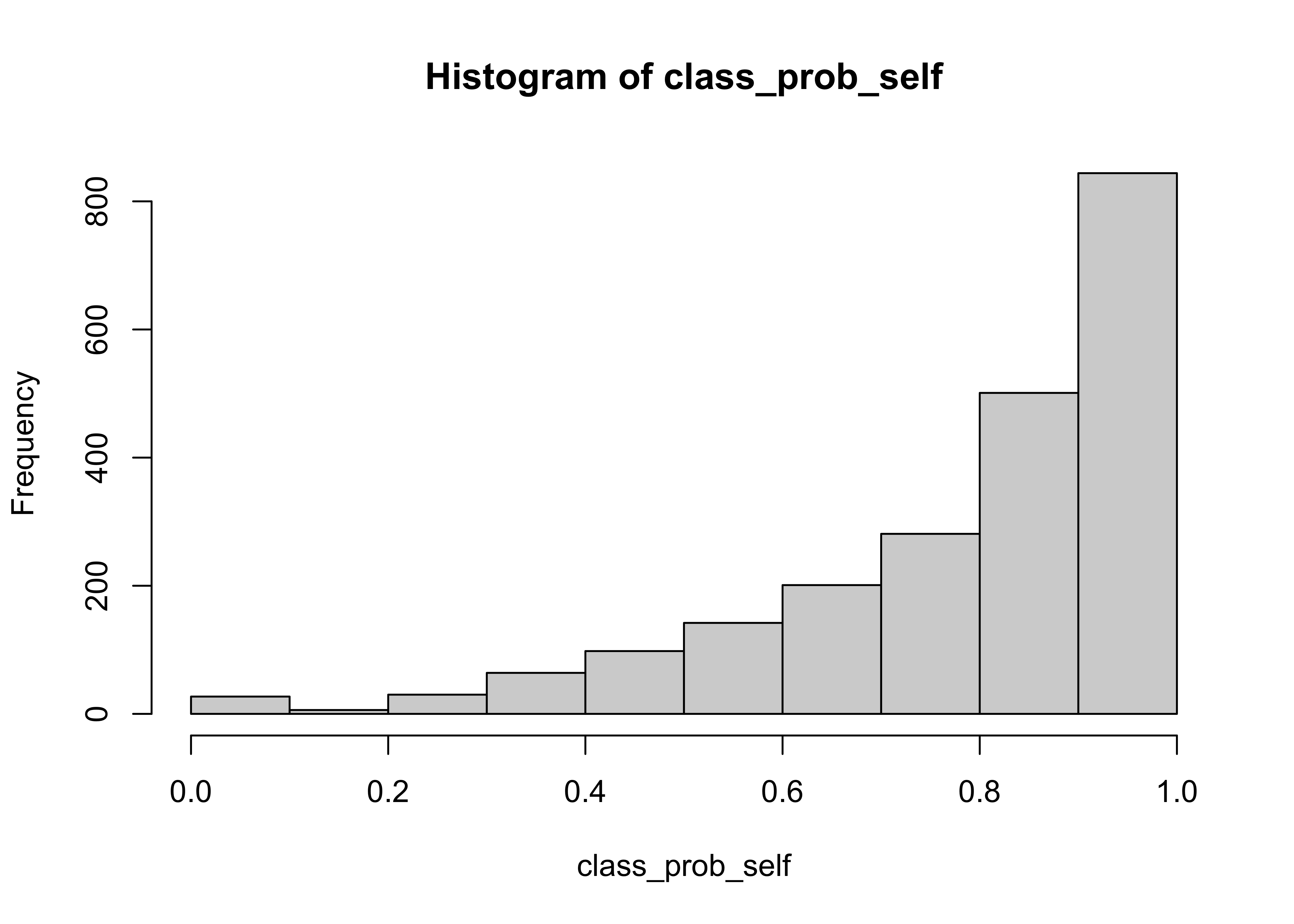
This means that even though the mean of the predicted probabilities (0.789) matches the proportion of self reported turnout in the data (0.789), if we use the 0.5 cutoff a higher proportion (0.897) are predicted to be voters. This illustrates nicely how using the point predictions based on some threshold instead of the predicted probabilities will introduce more bias.
- Repeat the steps 1-3 of Q4, but this time training on the validated turnout data
turnout_validated. You do not need to write up any discussion, just calculate the corresponding quantities inR. What is the correlation between the probability predictions based on training using self-reports and based on training using validated turnout? If we look at the binary predictions, what proportion of respondents get each of the four possible combinations of predictions from each of the two models? Note: Usenewdata=besinpredict()so that you construct fitted values for all observations (otherwise you will not get predictions for observations dropped due to missingturnout_validated).
# fit model
glm_fit_validated <- glm(turnout_validated~c02_1+c02_2+c02_3+c02_4,
                         data=bes,family=binomial(link = "logit"))

# construct probability predictions
class_prob_validated <- predict(glm_fit_validated,
                                newdata = bes,
                                type="response")

# construct dichotomous predictions
class_binary_validated <- class_prob_validated > 0.5

# correlation between predicted prob from the two models
cor(class_prob_self,class_prob_validated)
## [1] 0.9427171## class_binary_validated
## class_binary_self FALSE TRUE
## FALSE 0.08 0.02
## TRUE 0.03 0.87The probability predictions are highly correlated (0.94), but the binary classifications include a fair number of differently classified individuals (5%), at least relative to the total number of correctly predicted non-voters (8%). This happens because both models struggle to classify anyone as below 0.5, and so most such individuals are edge cases, and the different predictions of the two models (trained on similar, but different training data) make different point predictions about a substantial proportion of the predicted non-voters.
- Create confusion matrices for your two models. Calculate the total error rate, sensitivity and specificity of each model.
##        m
## mu      FALSE TRUE
##   FALSE   140  322
##   TRUE     85 1647
# confusion matrix model turnout_validated
cm2 <- table("mu"=bes$turnout_validated,"m"=class_binary_validated)
cm2## m
## mu FALSE TRUE
## FALSE 90 290
## TRUE 52 1043# Total error rate
## turnout_self
## this adds the proportions in the off-diagonals
te1 <- (cm1[2,1]+cm1[1,2])/sum(cm1)
## turnout_validated
te2 <- (cm2[2,1]+cm2[1,2])/sum(cm2)
# Sensitivity (for mu = 1)
## turnout_self
se1 <- cm1[2,2]/sum(cm1[2,])
## turnout_validated
se2 <- cm2[2,2]/sum(cm2[2,])
# Specificity (for mu = 0)
## turnout_self
sp1 <- cm1[1,1]/sum(cm1[1,])
## turnout_validated
sp2 <- cm2[1,1]/sum(cm2[1,])
# You could just look at the numbers one by one in the console,
# but you can also combine these in a nice table
tmp <- round(data.frame("Self-reported turnout" = c(te1,se1,sp1),
"Validated turnout" = c(te2,se2,sp2)),2)
rownames(tmp) <- c("Total error rate","Sensitivity","Specificity")
tmp## Self.reported.turnout Validated.turnout
## Total error rate 0.19 0.23
## Sensitivity 0.95 0.95
## Specificity 0.30 0.24The total error rate is about 18% for the turnout_self model and 23%, so slightly higher, for turnout_validated. This suggests that the predictors we used are slightly better at explaining why someone reported that they voted, rather than actually voting.
As is consistent with our discussion about the high rate of (self reported) voters in the training data above, the sensitivity (the rate of true positives) is quite high for both models. Interestingly, the model based on self reported turnout as the training data yields slightly higher specificity, meaning that the model here is slightly better at ‘catching’ true negatives.
7.2 Quiz
- When should one apply class measurement instead of scale measurement?
- When the target concept is binary or categorical.
- When there is a pre-existing, but binary ‘gold standard’ measure available.
- There are no ‘rules’ about when to measure classes rather than scales, it is a choice of the analyst.
- When we have a scale measure that we can split into categories according to meaningful thresholds.
- What is deductive reasoning?
- It is when we use observations for make generalisations (inferences) about a wider population and develop theoretical meaning based on these.
- It is another term for supervised measurement.
- It is another term for unsupervised measurement.
- It is when we use theory to derive predictions (hypotheses) which we use to draw conclusions about observations.
- Which of the following is not true about coding rules?
- When developing coding rules to link a categorical quantity to observable indicators, stronger supervision is better.
- Coding rules are necessarily context-specific as they are meant to encode substantive expertise.
- Coding rules are useless when dealing with ambiguous or borderline cases.
- Coding rules are generally developed via deductive reasoning.
- What do we need to worry about when assessing the usefulness of a supervised class measurement approach with logistic regression?
- The degree to which the associations between the indicators and \(\mu\) in the training set are representative of the associations in the target population.
- The availability and quality of the gold standard measure \(m\) and the degree to which it captures \(\mu\).
- How much variance in \(m\) the indicators account for and whether the unexplained variance is associated with \(\mu\).
- We should worry about all of these things, in the same way than we would in the context of interval-level scales.
- Which of the following is not true about logistic regression?
- The regression coefficients represent the linear effect of the independent variable X on the probability that Y=1.
- The regression equation \(\alpha + \beta_1\times X_1 + …\) gives you the predicted log-odds that \(Y=1\).
- The inverse logit of the regression equation \(\alpha + \beta_1\times X_1 + …\) gives you the predicted probability that \(Y=1\).
- The predicted probability that unit \(i\) is 1 incorporates uncertainty about the true value/classification of \(i\).
- Which of the following is the rate at which the true value is 1, when the model predicts a value of 1?
- Sensitivity
- Specificity
- Positive Predictive Value
- Negative Predictive Value