5 Supervised Scale Measurement II: Regression
Topics: Strategies for scale development with training data. Predictive modelling as measurement. Scales as linear functions of indicators. Estimating weights using training / “gold standard” data.
Required reading:
- Chapter 8, Pragmatic Social Measurement
Further reading:
Theory
Applications
- Where-to-be-born Index (The Economist Intelligence Unit)
- Pew Research Center, “Can Likely Voter Models Be Improved?? 2. Measuring the likelihood to vote”
- Pourghasemi, H.R., Moradi, H.R. & Fatemi Aghda, S.M. Landslide susceptibility mapping by binary logistic regression, analytical hierarchy process, and statistical index models and assessment of their performances. Nat Hazards 69, 749–779 (2013).
5.1 Seminar
This assignment follows the strategy used by the Economist Intelligence Unit’s “Where-to-be-born” index which aims to measure which countries tend to have the highest life satisfaction and therefore where you would want to be born in the “lottery of life”. The procedure followed by the Economist in 2006 was to start with data on the average life satisfaction in 130 countries, as measured by the Gallup World Poll. The Gallup prompt is:
Please imagine a ladder with steps numbered from zero at the bottom to 10 at the top. Suppose we say that the top of the ladder represents the best possible life for you, and the bottom of the ladder represents the worst possible life for you. On which step of the ladder would you say you personally feel you stand at this time, assuming that the higher the step the better you feel about your life, and the lower the step the worse you feel about it? Which step comes closest to the way you feel?
The Economist then used a multivariate regression to predict the country-level averages—the training data—as a function of a set of indicators:
“The life satisfaction scores for 2006 (on scale of 1 to 10) for 130 countries (from the Gallup Poll) are related in a multivariate regression to various factors. As many as 11 indicators are statistically significant. Together these indicators explain some 85% of the inter-country variation in life satisfaction scores. The values of the life satisfaction scores that are predicted by our indicators represent a country’s quality of life index. The coefficients in the estimated equation weight automatically the importance of the various factors. We can utilise the estimated equation for 2006 to calculate index values for year in the past and future, allowing for comparison over time as well across countries.
“The independent variables in the estimating equation for 2006 include: material wellbeing as measured by GDP per head (in $, at 2006 constant PPPS); life expectancy at birth; the quality of family life, based primarily on divorce rates; the state of political freedoms; job security (measured by the unemployment rate); climate (measured by two variables: the average deviation of minimum and maximum monthly temperatures from 14 degrees Celsius; and the number of months in the year with less than 30mm rainfall); personal physical security ratings (based primarily on recorded homicide rates and ratings for risk from crime and terrorism); quality of community life (based on membership in social organisations); governance (measured by ratings for corruption); gender equality (measured by the share of seats in parliament held by women).
“We find that GDP per head alone explains some two thirds of the inter-country variation in life satisfaction, and the estimated relationship is linear. Surveys show that, even in rich countries, people with higher incomes are more satisfied with life than those with lower incomes. However, over several decades there has been only a very modest upward trend in average life satisfaction scores in developed nations, whereas average income has grown substantially. The explanation is that there are factors associated with development that, in part, offset the positive impact. A concomitant breakdown of traditional institutions is manifested in the decline of religiosity and of trade unions; a marked rise in various social pathologies (crime, drug and alcohol addiction); a decline in political participation and of trust in public authority; and the erosion of the institutions of family and marriage.” https://www.economist.com/news/2012/11/21/the-lottery-of-life-methodology
The Economist has been continuing to use the relationships estimated from the 2006 data to update their estimates.
In this week’s exercise, we are going to “re-train” the model using more recent 2014-16 data from Gallup. It is entirely possible that life satisfaction has a different relationship to various possible indicators than it did in 2006. We are not going to examine the same indicators here, mostly because some of them are difficult to collect. Instead, we are going to use the four indicators from the 2018 Human Development Index: life expectancy at birth (LE), expected years of schooling (EYS), mean years of schooling (MYS), and GNI per capita (GNI). The variable LifeSat gives the average life satisfaction as measured by Gallup (2014-16).
- Use
ggpairs()from the packageGGallyto plotLifeSatand the four indicatorsLE,EYS,MYSandlog(GNI)against one another and their pairwise correlations.
# install.packages("GGally")
library(GGally)
lifesat_df$logGNI <- log(lifesat_df$GNI)
ggpairs(lifesat_df, columns = c(3,7:9,11))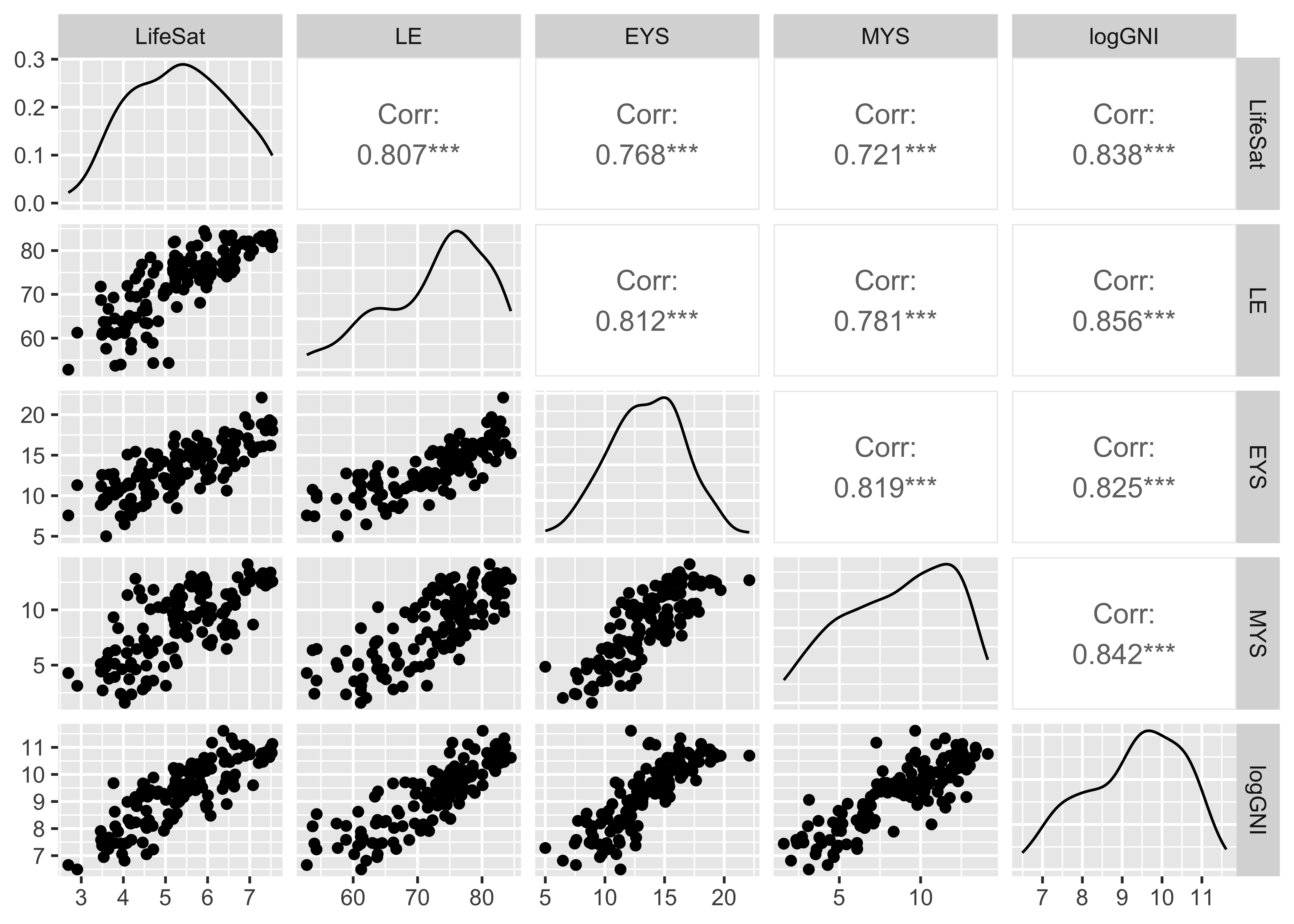
All of these variables are highly correlated with one another, with correlation coefficients ranging from 0.72 (LifeSat with MYS) to 0.86 (LE with log(GNI)).
- Fit a linear regression predicting
LifeSatwith the four indicatorsLE,EYS,MYSandlog(GNI). Which of the country-level indicators most strongly predict country-level life satisfaction? Which of the country-level indicators do not predict country-level life satisfaction well, or have coefficients that seem to make less substantive sense?
##
## =======================
##              Model 1
## -----------------------
## (Intercept)   -2.94 ***
##               (0.67)
## LE             0.04 **
##               (0.01)
## EYS            0.07
##               (0.03)
## MYS           -0.03
##               (0.03)
## log(GNI)       0.50 ***
##               (0.10)
## -----------------------
## R^2            0.74
## Adj. R^2       0.73
## Num. obs.    134
## =======================
## *** p < 0.001; ** p < 0.01; * p < 0.05
Of the four indicators, log(GNI) has the largest coefficient in the model that includes all four. As we saw above in Q1, all four indicators are individually quite predictive of life satisfaction, but once they are all included in a model together, some of them are no longer conditionally predictive given the information in the other indicators.
- The expected years of schooling (EYS) and mean years of schooling are highly collinear (\(r\) = 0.82, and largely measure the same concept. Drop the one whose coefficient in the initial makes less substantive sense, and refit the linear regression.
##
## =======================
##              Model 1
## -----------------------
## (Intercept)   -2.64 ***
##               (0.57)
## LE             0.04 **
##               (0.01)
## EYS            0.05
##               (0.03)
## log(GNI)       0.47 ***
##               (0.09)
## -----------------------
## R^2            0.74
## Adj. R^2       0.73
## Num. obs.    134
## =======================
## *** p < 0.001; ** p < 0.01; * p < 0.05
I drop MYS, which had a negative (but insignificant) coefficient in the model we fit in Q2. There is no reason to expect this measure of schooling to be associated with reduced life satisfaction, and given that it had an insignificant partial association and is a similar measure to EYS, it is the obvious candidate to drop. That said, the model changes very little when we drop it, because it had a negligible coefficient when included.
- The data set includes
HDI, which is calculated from these same indicators (look ahead to next week’s chapter of the textbook for details). How highly correlated are the fitted values from the regression that we just fit withHDI? How highly correlated isLifeSatwithHDI? Explain the difference between these two correlations (this does not require looking up how HDI is calculated from the indicators).
## [1] 0.9890412## [1] 0.8428343The fitted values from the regression are correlated with HDI at 0.99, while the original LifeSat variable is correlated with HDI at 0.84. The fitted values are more highly correlated because they use the same indicators as HDI, they can only differ from HDI to the extent to which those indicators are aggregated in a different ways (different functional form, different coefficients). The original life satisfaction measures from Gallup can vary for many reasons beyond those captured by these indicators; the fitted values are constructed from the indicators and can only vary with them.
This is more a mechanical result of the way that the different quantities are constructed rather than something profound, however the fact that the fitted value are so highly correlated with HDI does indicate that the way HDI aggregates the indicators is very similar to how our model trained on life satisfaction data aggregates the indicators, which is interesting.
- What are the largest positive and negative residuals in the training data? That is, which country has a Gallup measured life satisfaction that most exceeds what the fitted model predicts? Which country falls furthest below what the model predicts? Compare the indicator profiles, HDI and LifeSat for these two countries.
## [1] "Guatemala"## [1] "Botswana"## X Name LifeSat CountryCode Region HDI LE
## 18 18 Botswana 3.766 BWA Sub-Saharan Africa 0.7277871 69.275
## 48 48 Guatemala 6.454 GTM Latin America & Caribbean 0.6510353 74.063
## EYS MYS GNI logGNI
## 18 12.69723 9.330000 15951.330 9.677298
## 48 10.62148 6.467886 7377.916 8.906246The largest positive residual is Guatemala, the largest negative residual is Botswana. Guatemala has measured life satisfaction slightly above France and Spain, which outrank it substantially in terms of HDI / the fitted model. Botswana, despite higher educational attainment than Guatemala and twice the GNI per capita, has far lower life satisfaction, among the lowest of any country in the data. Guatemala does have higher life expectancy than Botswana by 5 years, but nonetheless has lower HDI and a lower fitted value from our life satisfaction model.
- Add
Regionto the linear regression model. Does it improve the fit of the model? Which regions have higher/lower levels of life satisfaction, holding constant the other indicators?
##
## ============================================
##                                   Model 1
## --------------------------------------------
## (Intercept)                        -2.57 **
##                                    (0.95)
## LE                                  0.03
##                                    (0.02)
## EYS                                 0.06
##                                    (0.03)
## log(GNI)                            0.55 ***
##                                    (0.09)
## RegionEurope & Central Asia        -0.14
##                                    (0.19)
## RegionLatin America & Caribbean     0.60 **
##                                    (0.21)
## RegionMiddle East & North Africa   -0.12
##                                    (0.22)
## RegionNorth America                 0.60
##                                    (0.44)
## RegionSouth Asia                   -0.09
##                                    (0.28)
## RegionSub-Saharan Africa           -0.01
##                                    (0.25)
## --------------------------------------------
## R^2                                 0.78
## Adj. R^2                            0.77
## Num. obs.                         134
## ============================================
## *** p < 0.001; ** p < 0.01; * p < 0.05
Region slightly improves the fit of the model. Countries in Latin America and the Caribbean appear to report higher life satisfaction at the same levels of life expectancy, schooling and GNI than countries in other regions. North America has the same positive coefficient, but very few countries, and thus is not statistically different from the baseline region (East Asia & Pacific).
- Do you think it makes sense to include a variable like
Regionin this kind of measurement model? What are some arguments for or against?
Whether we want to include region or not may depend on our aims. Countries cannot change their region. If our aim is to build a measure that captures the contributions of concrete quality of life variables like life expectancy, schooling and income to human life satisfaction, with an eye towards tracking changes over time (as the original analysis by the Economist did), we might not want to include a variable like region.
However, we might also view region as functioning as a proxy for other inputs, like climate, that might have real causal effects on human life satisfaction, even if they are (largely) out of the control of societies to change. The original aim of the Economist’s analysis was to assess where you would want to be born in the “lottery of life”. If people are just happier in some places, even if not for reasons we completely understand, that does seem relevant to the concept that the Economist wanted to measure. While you can imagine direct causal effects of things like life expectancy, schooling and national income, whereas region is more clearly a proxy for other things, in reality these indicators are all proxies for much more complex underlying causal processes, and it is difficult to imagine narrow manipulations of any of them.
- The Economist’s original measurement strategy was to calibrate the relationships between their indicators and country-level life satisfaction once (using data from 2006), and then use the resulting model with updated indicators in the future, without recalibrating on newer life satisfaction survey data. What is the key implicit assumption required for this to be a good measurement strategy?
Narrowly stated, the key assumption is that, if you re-ran the calibration exercise with new life satisfaction survey data, you would find the same coefficients on the indicators. That is to say, in the same set of countries, the relationship between life satisfaction and the various indicators has to be stable, such that when we see the indicators change, we also see life satisfaction change according to the model. Note that this is a strong causal assumption about the relationship between the indicators and life satisfaction, for which neither we nor the Economist have any evidence.
5.2 Quiz
- What is supervised measurement?
- It refers to cases where we only have observable data about indicators and use covariation between them to discover relevant underlying concepts.
- It refers to cases where we have indicators which we think indicate something about the level/presence/absence of the target concept.
- It refers to cases where we use our substantive knowledge of and/or data about the relationship between concept and indicators to connect the two.
- It refers to cases where we have good quality training data on which we can build a measurement model.
- Which of the following is not true about the use of regression in the context of supervised scale measurement?
- The main goal is predictive performance.
- Not everyone has the same number of matches.
- We need to have data about the gold standard measure m for the training units and have data about at least one indicator for both the training units and those we seek to apply the measurement to.
- The main goal is to minimise the training error rate.
- The main goal is to jointly maximise reliability and validity (= jointly minimise bias and variance).
- What are things we do not need to worry about when assessing the usefulness of a supervised measurement design with regression?
- The degree to which the associations between the indicators and \(\mu\) in the training set are representative of the associations in the target population.
- The quality of the gold standard measure m and the degree to which it captures \(\mu\).
- How much variance in m the indicators account for and whether the unexplained variance is associated with \(\mu\).
- We should worry about all of these things.
- That the coefficients for all indicators are statistically significant.
- When is this approach particularly useful?
- Where the training set (and the gold measure m) is cheap to construct.
- When we want to measure something that may or may not happen in the future in the present.
- When we don’t have any data related to our target concept of interest.
- When we don’t have any indicator data for our target population, but only for the training data.