9 Topic Models
9.1 Seminar
9.1.1 Exercise
Load the necessary packages up front.
library(quanteda)
library(quantedaData)
library(readtext)

library(tidyverse)
Load the fake-news data from Kaggle and create a corpus object using quanteda.
fake_news <- readtext("https://uclspp.github.io/datasets/data/fake-news.zip",
                      text_field = "text")

fake_news_corpus = corpus(fake_news)
Create a document-feature matrix using dfm. Remove tokens that appear infrequently and those less than 4 characters long.
fake_news_dfm <- dfm(fake_news_corpus,
                stem = TRUE,
                remove = stopwords("SMART"),
                remove_punct = TRUE,
                remove_numbers = TRUE)
Warning: 'stopwords(language = "SMART")' is deprecated.
Use 'stopwords(source = "smart")' instead.
See help("Deprecated")fake_news_dfm <- dfm_trim(fake_news_dfm, min_count = 10, min_docfreq = 5)
fake_news_dfm <- dfm_select(fake_news_dfm, min_nchar = 4)Using topicmodels Package
library(topicmodels)
library(tidytext)
Convert the document-feature matrix to the format that the topicmodels package requires.
fake_news_dtm_topicmodels <- convert(fake_news_dfm, to = "topicmodels")Fit a topic model using LDA. Wrapping your code inside system.time will tell you how long it took to run.
system.time(
  topic_model <- LDA(fake_news_dtm_topicmodels, k = 4)
)
user system elapsed
448.964 0.588 449.622 Get topic proportions for each document.
posterior_probs <- posterior(topic_model)
topic_proportions <- as.data.frame(posterior_probs$topics)

# show topic proportions for first 10 documents
head(topic_proportions, n = 10)
1 2 3 4
text1 0.0026802877 0.0026805035 0.5972145 0.3974246880
text2 0.0006370018 0.0006370317 0.8612489 0.1374770259
text3 0.0010118949 0.0010119414 0.9969642 0.0010119426
text4 0.0036705725 0.0036708808 0.9889876 0.0036709545
text5 0.0005646082 0.7096049318 0.2892658 0.0005646300
text6 0.0008998546 0.0008999118 0.9973003 0.0008998991
text7 0.0002338378 0.0002338511 0.9992985 0.0002338476
text8 0.0004418409 0.0295411333 0.9695752 0.0004418431
text9 0.0008908851 0.0008909248 0.9973273 0.0008909124
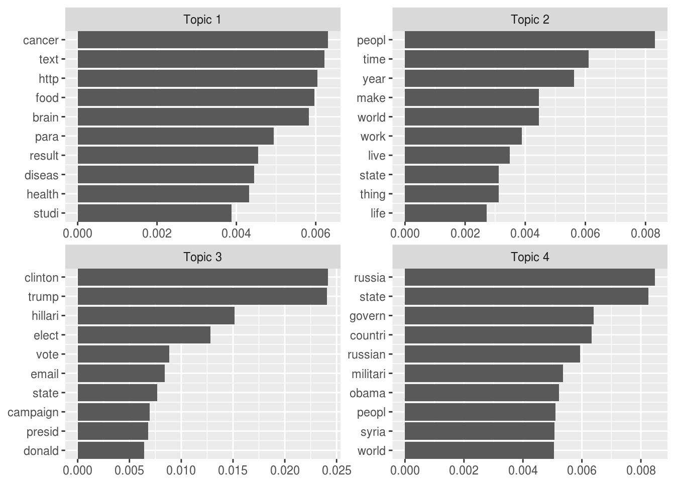
text10 0.0020156010 0.7395633852 0.2306829 0.0277380697Get the top 10 words from each topic
topic_terms <- tidy(topic_model) %>%
  mutate(topic = paste("Topic", topic)) %>%
  group_by(topic) %>%
  mutate(term = reorder(term, desc(beta))) %>%
  top_n(10, beta) %>%
  ungroup() %>%
  arrange(topic, desc(beta)) %>%
  mutate(order = row_number())
Plot the words using ggplot
ggplot(topic_terms, aes(order, beta)) +
  geom_bar(stat = "identity", show.legend = FALSE) +
  facet_wrap(~topic, scales = "free") +
  coord_flip() +
  scale_x_continuous(
    trans = "reverse",
    breaks = topic_terms$order,
    labels = topic_terms$term,
    expand = c(0,0)
  ) +
  theme(
    axis.title = element_blank()
  )
Using lda Package with LDAvis
library(lda)
library(LDAvis)
Convert the document-feature matrix to the format that the lda package requires.
fake_news_dtm_lda <- convert(fake_news_dfm, to = "lda")Fit a topic model using LDA.
set.seed(12345)

alpha <- 0.02
eta <- 0.02

# you can reduce the number of iterations if it takes too long to run

system.time(
  topic_model <- lda.collapsed.gibbs.sampler(documents = fake_news_dtm_lda$documents,
                                             K = 20,
                                             alpha = alpha,
                                             eta = eta,
                                             vocab = fake_news_dtm_lda$vocab,
                                             num.iterations = 500,
                                             initial = NULL,
                                             burnin = 0,
                                             compute.log.likelihood = TRUE)
)
user system elapsed
487.800 0.040 487.903 Extarct the phi and theta parameters from the trained model.
phi <- t(apply(topic_model$topics + eta, 1, function(x) x/sum(x)))
theta <- t(apply(topic_model$document_sums + alpha, 2, function(x) x/sum(x)))
We also need to find the number of tokens in each document.
doc_length <- sapply(fake_news_dtm_lda$documents, function(x) { sum(x[2,]) })Crete a JSON object for our visualization.
json_vis <- createJSON(phi = phi,
                       theta = theta,
                       doc.length = doc_length,
                       vocab = fake_news_dtm_lda$vocab,
                       term.frequency = colSums(fake_news_dfm))
Run the visualization server. You should see a topic model in either the viewer tab or in a separate browser window. You can stop the server by pressing the ESC key on the keyboard.
serVis(json_vis, open.browser = TRUE)