4.2 Solutions
You will need to load the core library for the course textbook:
Let’s load all the packages upfront. NOTE: we use message=FALSE to suppress some messages.
library(ISLR)
library(MASS)
library(glmnet)
library(leaps)
library(pls)
4.2.1 Exercise
In the lab session for this topic (Sections 5.3.2 and 5.3.3 in James et al.), we saw that the cv.glm() function can be used in order to compute the LOOCV test error estimate. Alternatively, one could compute those quantities using just the glm() and predict.glm() functions, and a for loop. You will now take this approach in order to compute the LOOCV error for a simple logistic regression model on the Weekly data set. Recall that in the context of classification problems, the LOOCV error is given in Section 5.1.5 (5.4, page 184).
- Fit a logistic regression model that predicts
DirectionusingLag1andLag2.
logit_model <- glm(Direction ~ Lag1 + Lag2, data = Weekly, family = binomial)
summary(logit_model)
Call:
glm(formula = Direction ~ Lag1 + Lag2, family = binomial, data = Weekly)

Deviance Residuals:
   Min      1Q  Median      3Q     Max
-1.623  -1.261   1.001   1.083   1.506

Coefficients:
            Estimate Std. Error z value Pr(>|z|)
(Intercept)  0.22122    0.06147   3.599 0.000319 ***
Lag1        -0.03872    0.02622  -1.477 0.139672
Lag2         0.06025    0.02655   2.270 0.023232 *
---
Signif. codes:  0 '***' 0.001 '**' 0.01 '*' 0.05 '.' 0.1 ' ' 1

(Dispersion parameter for binomial family taken to be 1)

    Null deviance: 1496.2  on 1088  degrees of freedom
Residual deviance: 1488.2  on 1086  degrees of freedom
AIC: 1494.2

Number of Fisher Scoring iterations: 4- Fit a logistic regression model that predicts
DirectionusingLag1andLag2using all but the first observation.
logit_model <- glm(Direction ~ Lag1 + Lag2, data = Weekly[-1,], family = binomial)
summary(logit_model)
Call:
glm(formula = Direction ~ Lag1 + Lag2, family = binomial, data = Weekly[-1,
    ])

Deviance Residuals:
    Min       1Q   Median       3Q      Max
-1.6258  -1.2617   0.9999   1.0819   1.5071

Coefficients:
            Estimate Std. Error z value Pr(>|z|)
(Intercept)  0.22324    0.06150   3.630 0.000283 ***
Lag1        -0.03843    0.02622  -1.466 0.142683
Lag2         0.06085    0.02656   2.291 0.021971 *
---
Signif. codes:  0 '***' 0.001 '**' 0.01 '*' 0.05 '.' 0.1 ' ' 1

(Dispersion parameter for binomial family taken to be 1)

    Null deviance: 1494.6  on 1087  degrees of freedom
Residual deviance: 1486.5  on 1085  degrees of freedom
AIC: 1492.5

Number of Fisher Scoring iterations: 4- Use the model from (b) to predict the direction of the first observation. You can do this by predicting that the first observation will go up if
P(Direction="Up"|Lag1, Lag2) > 0.5. Was this observation correctly classified?
Instead of writing the code all over the place that converts predicted probabilities to Up/Down, we’ll use a function similar to what we did last week.
# get prediction as Up/Down direction - same function as what we used last week
predict_glm_direction <- function(model, newdata = NULL) {
  predictions <- predict(model, newdata, type="response")
  return(ifelse(predictions < 0.5, "Down", "Up"))
}

predicted_direction <- predict_glm_direction(logit_model, Weekly[1,])
Prediction was Up, true direction was Down
Write a
forloop from i=1 to i=n, where n is the number of observations in the data set, that performs each of the following steps:Fit a logistic regression model using all but the i-th observation to predict
DirectionusingLag1andLag2.Compute the posterior probability of the market moving up for the i-th observation.
Use the posterior probability for the i-th observation in order to predict whether or not the market moves up.
Determine whether or not an error was made in predicting the direction for the i-th observation. If an error was made, then indicate this as a 1, and otherwise indicate it as a 0.
prediction_errors <-rep(NA, nrow(Weekly))

for (i in 1:nrow(Weekly)) {
   logit_model <- glm(Direction ~ Lag1 + Lag2, data = Weekly[-i,], family = binomial)

   predicted_direction <- predict_glm_direction(logit_model, Weekly[i,])

   prediction_errors[i] <- ifelse(predicted_direction != Weekly$Direction[i], 1, 0)
}- Take the average of the n numbers obtained in (d)iv in order to obtain the LOOCV estimate for the test error. Comment on the results.
mean(prediction_errors)[1] 0.4499541LOOCV estimates a test error rate of 0.4499541.
4.2.2 Exercise
In this exercise, we will predict the number of applications received using the other variables in the College data set.
- Split the data set into a training set and a test set.
Load and split the College data.
# split the dataset into training and test set with the split_ratio. Optionally set the random seed before splitting
# returns a list of two elements:
#    - first element is the training subset
#    - second elemet is the test subset
sample_split <- function(dataset, split_ratio, seed = NULL) {
  set.seed(seed)

  train_subset <- sample(nrow(dataset) * split_ratio)

  return(list(
    train = dataset[train_subset, ],
    test = dataset[-train_subset, ]
  ))
}

college_split <- sample_split(College, 0.7, seed = 12345)- Fit a linear model using least squares on the training set, and report the test error obtained.
ols_model <- lm(Apps ~ . , data = college_split$train)
ols_predictions <- predict(ols_model, college_split$test)
Since we need to calculate the MSE throughout this exercise, let’s write a function to do that.
calc_rmse <- function(y, y_hat) {
  return(sqrt(mean((y - y_hat)^2)))
}
Now we can calculate the MSE for the OLS model
ols_rmse <- calc_rmse(college_split$test$Apps, ols_predictions)Test RMSE for OLS is: 1188.832
- Fit a ridge regression model on the training set, with \(\lambda\) chosen by cross-validation. Report the test error obtained.
Pick \(\lambda\) using training subset and report error on test subset
train_matrix <- model.matrix(Apps ~ . , data = college_split$train)
test_matrix <- model.matrix(Apps ~ . , data = college_split$test)

grid <- 10 ^ seq(4, -2, length = 100)

ridge_model <- cv.glmnet(train_matrix, college_split$train$Apps, alpha = 0, lambda = grid, thresh = 1e-12)

ridge_predictions <- predict(ridge_model, test_matrix, s = ridge_model$lambda.min)

ridge_rmse <- calc_rmse(college_split$test$Apps, ridge_predictions)
Test RMSE for ridge model is: 1188.8145824
- Fit a lasso model on the training set, with \(\lambda\) chosen by cross-validation. Report the test error obtained, along with the number of non-zero coefficient estimates.
Pick \(\lambda\) using training subset and report error on test subset
lasso_model <- cv.glmnet(train_matrix, college_split$train$Apps, alpha = 1, lambda = grid, thresh = 1e-12)

lasso_predictions <- predict(lasso_model, test_matrix, s = lasso_model$lambda.min)

lasso_rmse <- calc_rmse(college_split$test$Apps, lasso_predictions)
Test RMSE for lasso model is: 1188.7994726
predict(lasso_model, s = lasso_model$lambda.min, type = "coefficients")19 x 1 sparse Matrix of class "dgCMatrix"
1
(Intercept) -601.38112596
(Intercept) .
PrivateYes -321.41076249
Accept 1.70685797
Enroll -1.35810665
Top10perc 45.45111099
Top25perc -15.88692306
F.Undergrad 0.09983028
P.Undergrad 0.01567394
Outstate -0.09222852
Room.Board 0.11816525
Books -0.04056782
Personal 0.05792203
PhD -5.56419852
Terminal -5.43103094
S.F.Ratio 21.59623616
perc.alumni 1.87814752
Expend 0.10806715
Grad.Rate 8.13596816- Fit a PCR model on the training set, with \(M\) chosen by cross-validation. Report the test error obtained, along with the value of \(M\) selected by cross-validation.
pcr_model <- pcr(Apps ~ . , data = college_split$train, scale = TRUE, validation = "CV")

validationplot(pcr_model, val.type = "MSEP")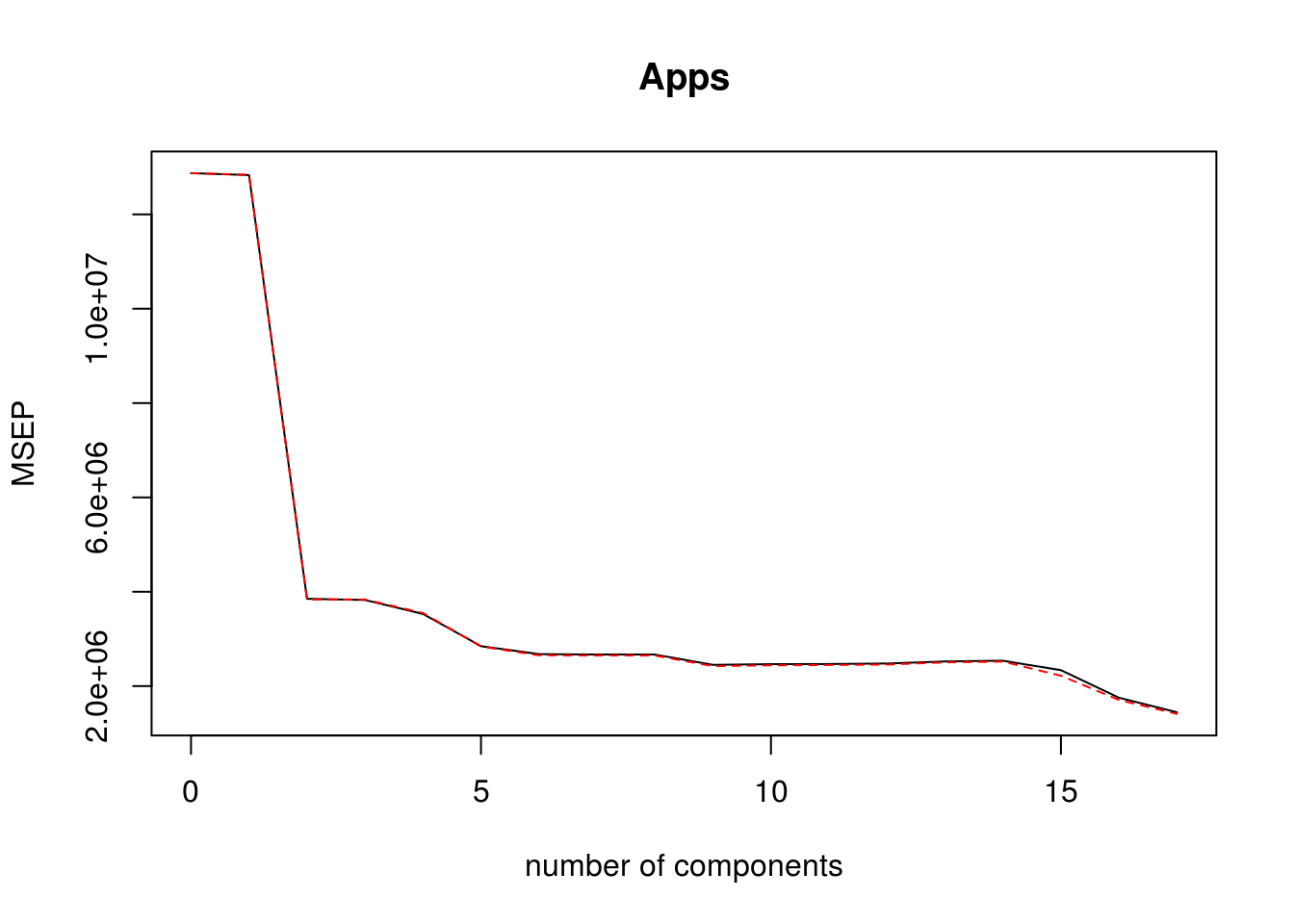
pcr_predictions <- predict(pcr_model, college_split$test, ncomp = 10)

pcr_rmse <- calc_rmse(college_split$test$Apps, pcr_predictions)
Test RMSE for PCR model is: 1556.8207088
- Fit a PLS model on the training set, with \(M\) chosen by cross-validation. Report the test error obtained, along with the value of \(M\) selected by cross-validation.
pls_model <- plsr(Apps ~ . , data = college_split$train, scale = TRUE, validation = "CV")

validationplot(pls_model, val.type = "MSEP")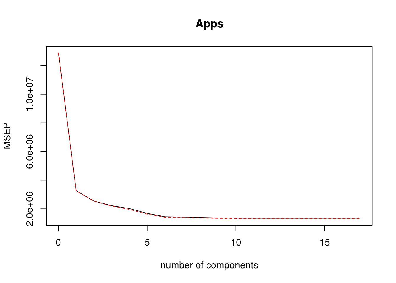
pls_predictions <- predict(pls_model, college_split$test, ncomp = 10)

pls_rmse <- calc_rmse(college_split$test$Apps, pls_predictions)
Test RMSE for PLS model is: 1178.3609154
- Comment on the results obtained. How accurately can we predict the number of college applications received? Is there much difference among the test errors resulting from these five approaches?
Let’s write a function to compute the \(R^2\) so we can compare the fit for various models. Recall that the \(R^2\) is given by:
\[R^2 = \frac{\mathrm{TSS - RSS}}{\mathrm{TSS}} = 1 - \frac{\mathrm{RSS}}{\mathrm{TSS}}\]
calc_r2 <- function(y, y_hat) {
  y_bar <- mean(y)
  rss <- sum((y - y_hat)^2)
  tss <- sum((y - y_bar)^2)
  return(1 - (rss / tss))
}
Results for OLS, Lasso, Ridge are comparable. Lasso reduces the \(F.Undergrad\) and \(Books\) variables to zero and shrinks coefficients of other variables. Here are the test \(R^2\) for all models.
ols_r2 <- calc_r2(college_split$test$Apps, ols_predictions)
ridge_r2 <- calc_r2(college_split$test$Apps, ridge_predictions)
lasso_r2 <- calc_r2(college_split$test$Apps, lasso_predictions)
pcr_r2 <- calc_r2(college_split$test$Apps, pcr_predictions)
pls_r2 <- calc_r2(college_split$test$Apps, pls_predictions)

barplot(c(ols_r2, ridge_r2, lasso_r2, pcr_r2, pls_r2),
        names.arg = c("OLS", "Ridge", "Lasso", "PCR", "PLS"))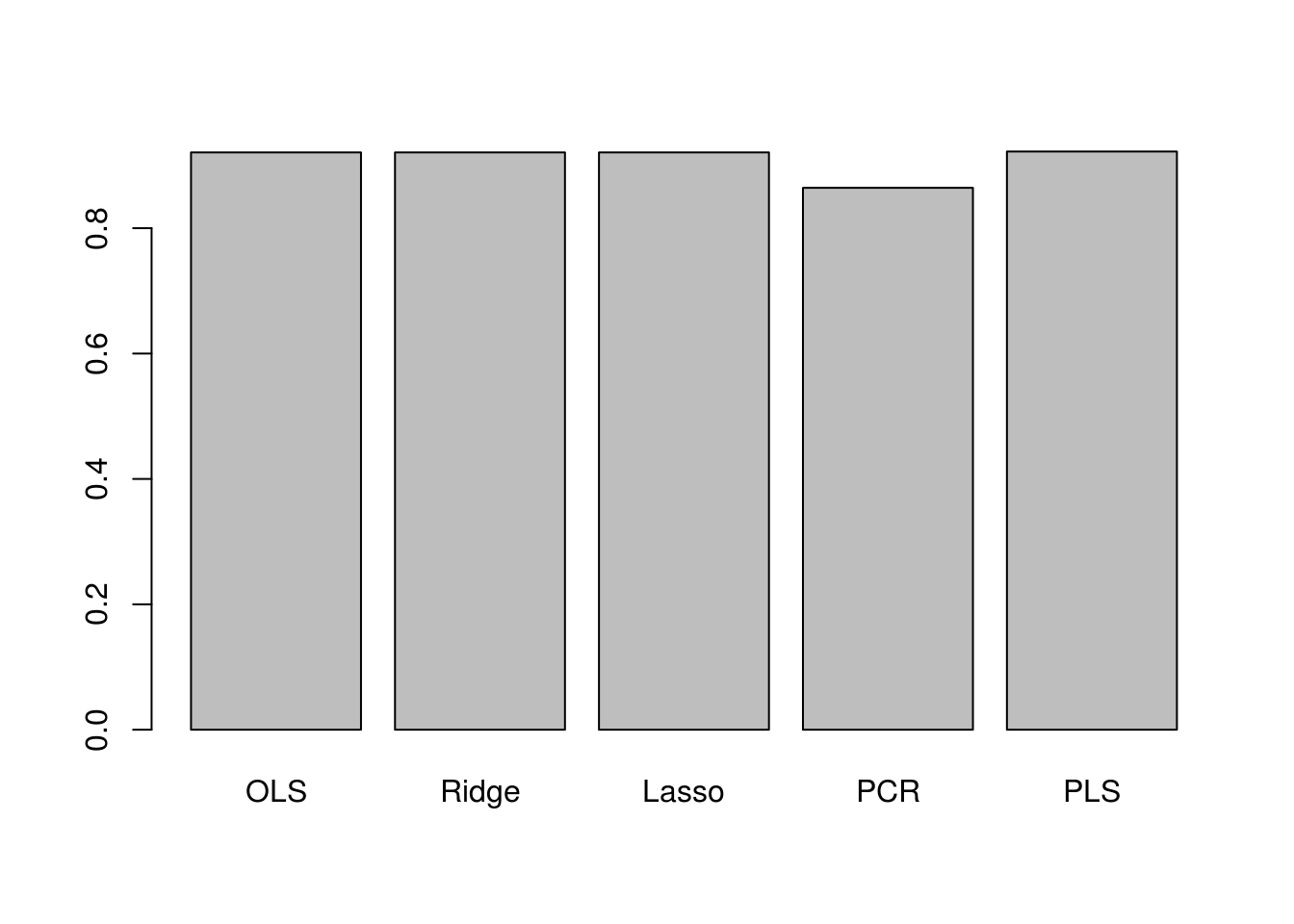
The plot shows that test \(R^2\) for all models except PCR are around 0.9, with PLS having slightly higher test \(R^2\) than others. PCR has a smaller test \(R^2\) of less than 0.8. All models except PCR predict college applications with high accuracy.
4.2.3 Exercise
We will now try to predict per capita crime rate in the Boston data set.
- Try out some of the regression methods explored in this chapter, such as best subset selection, the lasso, ridge regression, and PCR. Present and discuss results for the approaches that you consider.
Best subset selection
We need a function for getting predictions from a regsubsets model.
predict.regsubsets <- function(object, newdata, id, ...) {
  formula <- as.formula(object$call[[2]])
  model_matrix <- model.matrix(formula, newdata)
  coefi <- coef(object, id = id)
  model_matrix[, names(coefi)] %*% coefi
}
Now run K-fold cross-validation
set.seed(12345)

k <- 10
p <- ncol(Boston)-1
folds <- sample(rep(1:k, length = nrow(Boston)))
cv_errors <- matrix(NA, k, p)

for (i in 1:k) {
  best_fit <- regsubsets(crim ~ . , data = Boston[folds!=i,], nvmax = p)
  for (j in 1:p) {
    prediction <- predict(best_fit, Boston[folds==i, ], id = j)
    cv_errors[i,j] <-  mean((Boston$crim[folds==i] - prediction)^2)
  }
}

cv_rmse <- sqrt(apply(cv_errors, 2, mean))
plot(cv_rmse, type = "b")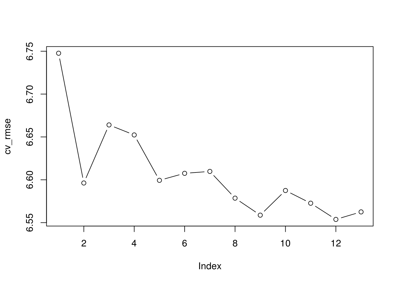
which.min(cv_rmse)[1] 12min(cv_rmse)[1] 6.55376Lasso
x <- model.matrix(crim ~ . -1, data = Boston)
cv_lasso <- cv.glmnet(x, Boston$crim, type.measure = "mse", alpha = 1)
plot(cv_lasso)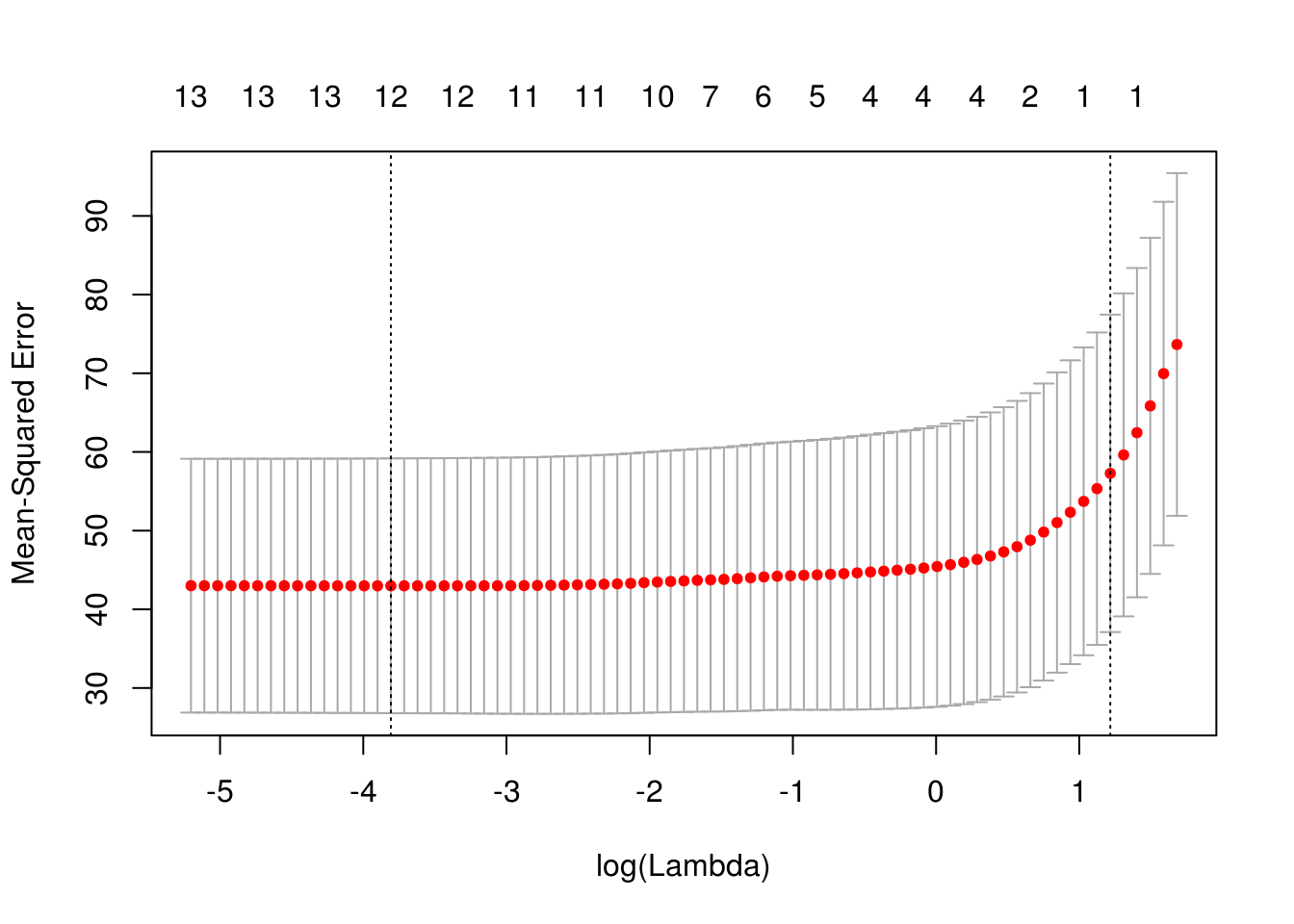
coef(cv_lasso)14 x 1 sparse Matrix of class "dgCMatrix"
1
(Intercept) 1.4186414
zn .
indus .
chas .
nox .
rm .
age .
dis .
rad 0.2298449
tax .
ptratio .
black .
lstat .
medv . sqrt(cv_lasso$cvm[cv_lasso$lambda == cv_lasso$lambda.1se])[1] 7.568515Ridge regression
x <- model.matrix(crim ~ . -1, data = Boston)
cv_ridge <- cv.glmnet(x, Boston$crim, type.measure = "mse", alpha = 0)
plot(cv_ridge)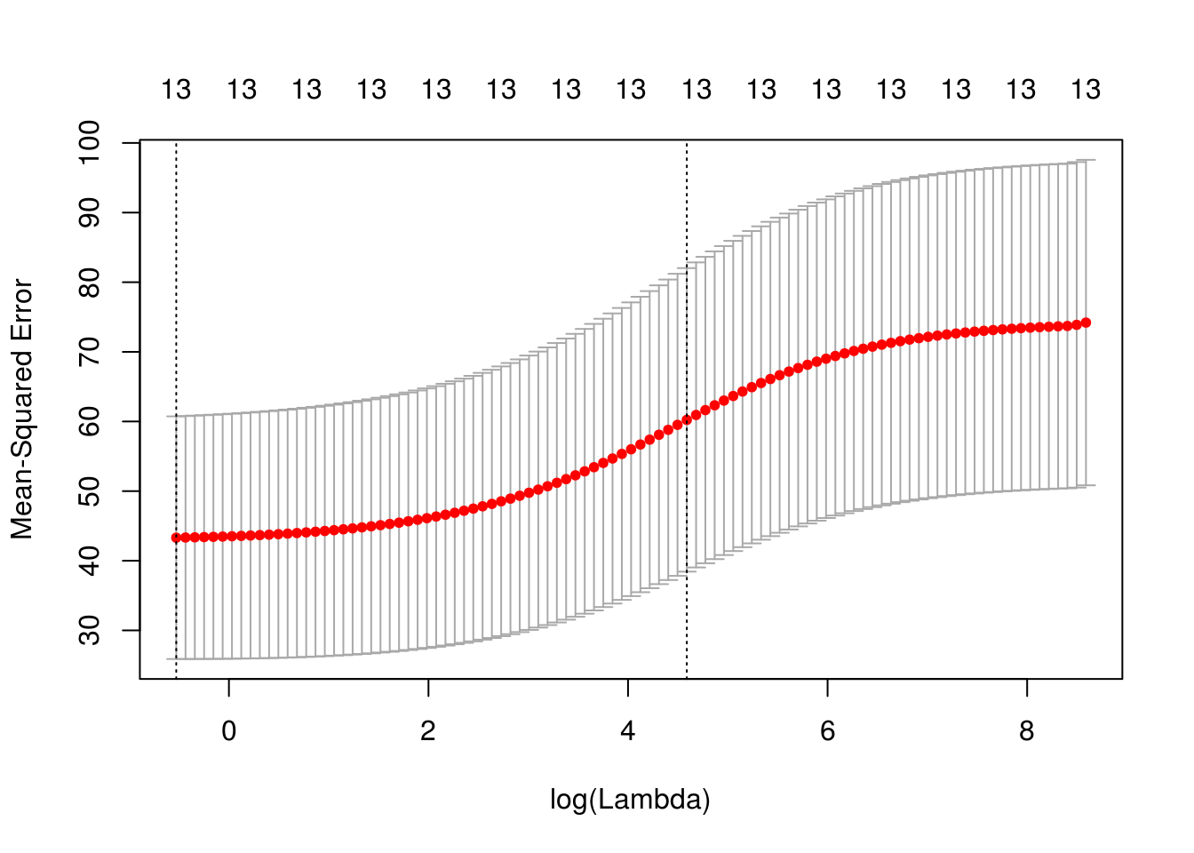
coef(cv_ridge)14 x 1 sparse Matrix of class "dgCMatrix"
1
(Intercept) 1.761587688
zn -0.002865786
indus 0.026514040
chas -0.142145708
nox 1.684835359
rm -0.130992458
age 0.005612849
dis -0.084630196
rad 0.039946869
tax 0.001830673
ptratio 0.063756646
black -0.002278831
lstat 0.031682619
medv -0.020839190sqrt(cv_ridge$cvm[cv_ridge$lambda == cv_ridge$lambda.1se])[1] 7.760891PCR
pcr_model <- pcr(crim ~ . , data = Boston, scale = TRUE, validation = "CV")
summary(pcr_model)
Data: X dimension: 506 13
Y dimension: 506 1
Fit method: svdpc
Number of components considered: 13
VALIDATION: RMSEP
Cross-validated using 10 random segments.
(Intercept) 1 comps 2 comps 3 comps 4 comps 5 comps 6 comps
CV 8.61 7.270 7.278 6.832 6.824 6.855 6.908
adjCV 8.61 7.264 7.272 6.824 6.813 6.846 6.895
7 comps 8 comps 9 comps 10 comps 11 comps 12 comps 13 comps
CV 6.901 6.770 6.800 6.795 6.811 6.784 6.705
adjCV 6.887 6.756 6.785 6.780 6.795 6.765 6.686
TRAINING: % variance explained
1 comps 2 comps 3 comps 4 comps 5 comps 6 comps 7 comps
X 47.70 60.36 69.67 76.45 82.99 88.00 91.14
crim 30.69 30.87 39.27 39.61 39.61 39.86 40.14
8 comps 9 comps 10 comps 11 comps 12 comps 13 comps
X 93.45 95.40 97.04 98.46 99.52 100.0
crim 42.47 42.55 42.78 43.04 44.13 45.413 component PCR fit has lowest CV/adjCV RMSEP.
- Propose a model (or set of models) that seem to perform well on this data set, and justify your answer. Make sure that you are evaluating model performance using validation set error, cross-validation, or some other reasonable alternative, as opposed to using training error.
See above answer for cross-validated mean squared errors of selected models.
- Does your chosen model involve all of the features in the data set? Why or why not?
I would choose the 12 parameter best subset model because it had the best cross-validated RMSE, next to PCR, but it was simpler model than the 13 component PCR model.