2.2 Solutions
library(ISLR)2.2.1 Exercise
This question involves the use of multiple linear regression on the Auto data set.
- Produce a scatterplot matrix which includes all of the variables in the data set.
pairs(Auto)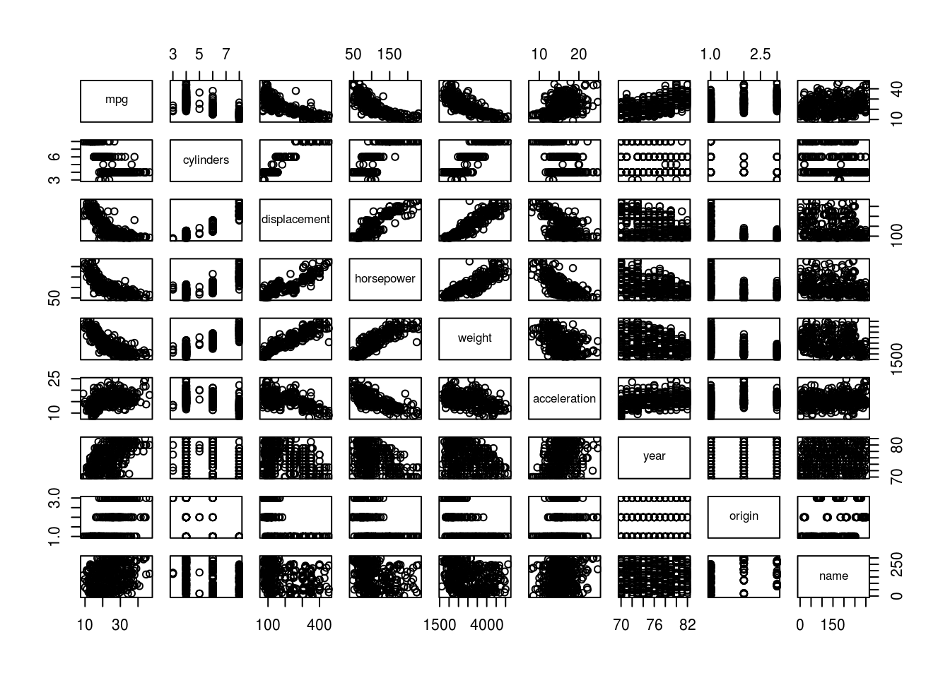
- Compute the matrix of correlations between the variables using the function
cor(). You will need to exclude thenamevariable, which is qualitative.
cor(subset(Auto, select = -name)) mpg cylinders displacement horsepower weight
mpg 1.0000000 -0.7776175 -0.8051269 -0.7784268 -0.8322442
cylinders -0.7776175 1.0000000 0.9508233 0.8429834 0.8975273
displacement -0.8051269 0.9508233 1.0000000 0.8972570 0.9329944
horsepower -0.7784268 0.8429834 0.8972570 1.0000000 0.8645377
weight -0.8322442 0.8975273 0.9329944 0.8645377 1.0000000
acceleration 0.4233285 -0.5046834 -0.5438005 -0.6891955 -0.4168392
year 0.5805410 -0.3456474 -0.3698552 -0.4163615 -0.3091199
origin 0.5652088 -0.5689316 -0.6145351 -0.4551715 -0.5850054
acceleration year origin
mpg 0.4233285 0.5805410 0.5652088
cylinders -0.5046834 -0.3456474 -0.5689316
displacement -0.5438005 -0.3698552 -0.6145351
horsepower -0.6891955 -0.4163615 -0.4551715
weight -0.4168392 -0.3091199 -0.5850054
acceleration 1.0000000 0.2903161 0.2127458
year 0.2903161 1.0000000 0.1815277
origin 0.2127458 0.1815277 1.0000000- Use the
lm()function to perform a multiple linear regression withmpgas the response and all other variables exceptnameas the predictors. Use thesummary()function to print the results. Comment on the output. For instance:
model1 <-  lm(mpg ~ .-name, data=Auto)
summary(model1)
Call:
lm(formula = mpg ~ . - name, data = Auto)

Residuals:
    Min      1Q  Median      3Q     Max
-9.5903 -2.1565 -0.1169  1.8690 13.0604

Coefficients:
               Estimate Std. Error t value Pr(>|t|)
(Intercept)  -17.218435   4.644294  -3.707  0.00024 ***
cylinders     -0.493376   0.323282  -1.526  0.12780
displacement   0.019896   0.007515   2.647  0.00844 **
horsepower    -0.016951   0.013787  -1.230  0.21963
weight        -0.006474   0.000652  -9.929  < 2e-16 ***
acceleration   0.080576   0.098845   0.815  0.41548
year           0.750773   0.050973  14.729  < 2e-16 ***
origin         1.426141   0.278136   5.127 4.67e-07 ***
---
Signif. codes:  0 '***' 0.001 '**' 0.01 '*' 0.05 '.' 0.1 ' ' 1

Residual standard error: 3.328 on 384 degrees of freedom
Multiple R-squared:  0.8215,    Adjusted R-squared:  0.8182
F-statistic: 252.4 on 7 and 384 DF,  p-value: < 2.2e-16
i. Is there a relationship between the predictors and the response?Yes, there is a relatioship between the predictors and the response by testing the null hypothesis of whether all the regression coefficients are zero. The F-statistic is far from 1 (with a small p-value), indicating evidence against the null hypothesis.
ii. Which predictors appear to have a statistically significant relationship to the response?Looking at the p-values associated with each predictor’s t-statistic, we see that displacement, weight, year, and origin have a statistically significant relationship, while cylinders, horsepower, and acceleration do not.
iii. What does the coefficient for the `year` variable suggest?The regression coefficient for year, 0.7507727, suggests that for every one year, mpg increases by the coefficient. In other words, cars become more fuel efficient every year by almost 1 mpg / year.
- Use the
plot()function to produce diagnostic plots of the linear regression fit. Comment on any problems you see with the fit. Do the residual plots suggest any unusually large outliers? Does the leverage plot identify any observations with unusually high leverage?
par(mfrow=c(2,2))
plot(model1)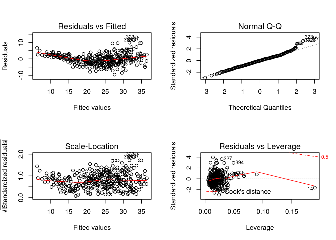
Seems to be non-linear pattern, linear model not the best fit. From the leverage plot, point 14 appears to have high leverage, although not a high magnitude residual.
plot(predict(model1), rstudent(model1))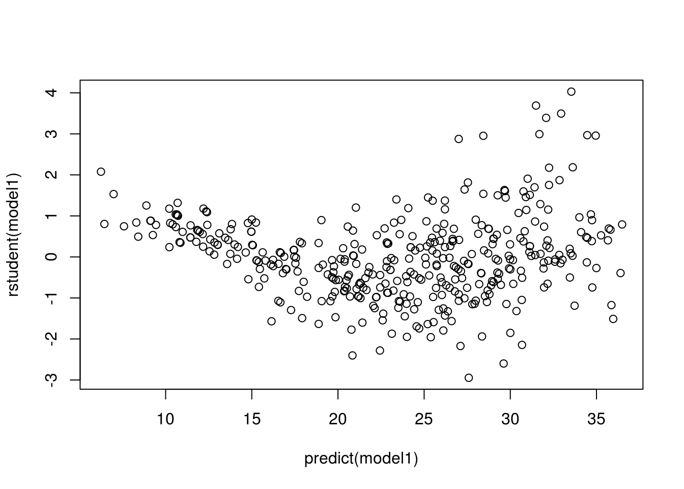
There are possible outliers as seen in the plot of studentized residuals because there are data with a value greater than 3.
- Use the
*and:symbols to fit linear regression models with interaction effects. Do any interactions appear to be statistically significant?
model2 <- lm(mpg ~ cylinders * displacement + displacement * weight, data=Auto)
summary(model2)
Call:
lm(formula = mpg ~ cylinders * displacement + displacement *
    weight, data = Auto)

Residuals:
     Min       1Q   Median       3Q      Max
-13.2934  -2.5184  -0.3476   1.8399  17.7723

Coefficients:
                         Estimate Std. Error t value Pr(>|t|)
(Intercept)             5.262e+01  2.237e+00  23.519  < 2e-16 ***
cylinders               7.606e-01  7.669e-01   0.992    0.322
displacement           -7.351e-02  1.669e-02  -4.403 1.38e-05 ***
weight                 -9.888e-03  1.329e-03  -7.438 6.69e-13 ***
cylinders:displacement -2.986e-03  3.426e-03  -0.872    0.384
displacement:weight     2.128e-05  5.002e-06   4.254 2.64e-05 ***
---
Signif. codes:  0 '***' 0.001 '**' 0.01 '*' 0.05 '.' 0.1 ' ' 1

Residual standard error: 4.103 on 386 degrees of freedom
Multiple R-squared:  0.7272,    Adjusted R-squared:  0.7237
F-statistic: 205.8 on 5 and 386 DF,  p-value: < 2.2e-16
Interaction between displacement and weight is statistically signifcant, while the interactiion between cylinders and displacement is not.
2.2.2 Exercise
This question should be answered using the Carseats dataset from the ISLR package.
- Fit a multiple regression model to predict
SalesusingPrice,Urban, andUS.
data(Carseats)
summary(Carseats)
Sales CompPrice Income Advertising
Min. : 0.000 Min. : 77 Min. : 21.00 Min. : 0.000
1st Qu.: 5.390 1st Qu.:115 1st Qu.: 42.75 1st Qu.: 0.000
Median : 7.490 Median :125 Median : 69.00 Median : 5.000
Mean : 7.496 Mean :125 Mean : 68.66 Mean : 6.635
3rd Qu.: 9.320 3rd Qu.:135 3rd Qu.: 91.00 3rd Qu.:12.000
Max. :16.270 Max. :175 Max. :120.00 Max. :29.000
Population Price ShelveLoc Age
Min. : 10.0 Min. : 24.0 Bad : 96 Min. :25.00
1st Qu.:139.0 1st Qu.:100.0 Good : 85 1st Qu.:39.75
Median :272.0 Median :117.0 Medium:219 Median :54.50
Mean :264.8 Mean :115.8 Mean :53.32
3rd Qu.:398.5 3rd Qu.:131.0 3rd Qu.:66.00
Max. :509.0 Max. :191.0 Max. :80.00
Education Urban US
Min. :10.0 No :118 No :142
1st Qu.:12.0 Yes:282 Yes:258
Median :14.0
Mean :13.9
3rd Qu.:16.0
Max. :18.0 model1 <- lm(Sales ~ Price + Urban + US, data = Carseats)
summary(model1)
Call:
lm(formula = Sales ~ Price + Urban + US, data = Carseats)

Residuals:
    Min      1Q  Median      3Q     Max
-6.9206 -1.6220 -0.0564  1.5786  7.0581

Coefficients:
             Estimate Std. Error t value Pr(>|t|)
(Intercept) 13.043469   0.651012  20.036  < 2e-16 ***
Price       -0.054459   0.005242 -10.389  < 2e-16 ***
UrbanYes    -0.021916   0.271650  -0.081    0.936
USYes        1.200573   0.259042   4.635 4.86e-06 ***
---
Signif. codes:  0 '***' 0.001 '**' 0.01 '*' 0.05 '.' 0.1 ' ' 1

Residual standard error: 2.472 on 396 degrees of freedom
Multiple R-squared:  0.2393,    Adjusted R-squared:  0.2335
F-statistic: 41.52 on 3 and 396 DF, p-value: < 2.2e-16- Provide an interpretation of each coefficient in the model. Be careful, some of the variables in the model are qualitative!
Price: suggests a relationship between price and sales given the low p-value of the t-statistic. The coefficient states a negative relationship between Price and Sales: as Price increases, Sales decreases.
UrbanYes: The linear regression suggests that there is not enough evidence for arelationship between the location of the store and the number of sales based.
USYes: Suggests there is a relationship between whether the store is in the US or not and the amount of sales. A positive relationship between USYes and Sales: if the store is in the US, the sales will increase by approximately 1201 units.
- Write out the model in equation form, being careful to handle the qualitative variables properly.
Sales = 13.04 + -0.05 Price + -0.02 UrbanYes + 1.20 USYes
- For which of the predictors can you reject the null hypothesis \(H_0 : \beta_j =0\)?
Price and USYes, based on the p-values, F-statistic, and p-value of the F-statistic.
- On the basis of your response to the previous question, fit a smaller model that only uses the predictors for which there is evidence of association with the outcome.
model2 <-  lm(Sales ~ Price + US, data = Carseats)
summary(model2)
Call:
lm(formula = Sales ~ Price + US, data = Carseats)

Residuals:
    Min      1Q  Median      3Q     Max
-6.9269 -1.6286 -0.0574  1.5766  7.0515

Coefficients:
            Estimate Std. Error t value Pr(>|t|)
(Intercept) 13.03079    0.63098  20.652  < 2e-16 ***
Price       -0.05448    0.00523 -10.416  < 2e-16 ***
USYes        1.19964    0.25846   4.641 4.71e-06 ***
---
Signif. codes:  0 '***' 0.001 '**' 0.01 '*' 0.05 '.' 0.1 ' ' 1

Residual standard error: 2.469 on 397 degrees of freedom
Multiple R-squared:  0.2393,    Adjusted R-squared:  0.2354
F-statistic: 62.43 on 2 and 397 DF, p-value: < 2.2e-16- How well do the models in (a) and (e) fit the data?
Based on the RSE and R^2 of the linear regressions, they both fit the data similarly, with linear regression from (e) fitting the data slightly better.
- Using the model from (e), obtain 95% confidence intervals for the coefficient(s).
confint(model2) 2.5 % 97.5 %
(Intercept) 11.79032020 14.27126531
Price -0.06475984 -0.04419543
USYes 0.69151957 1.70776632- Is there evidence of outliers or high leverage observations in the model from (e)?
plot(predict(model2), rstudent(model2))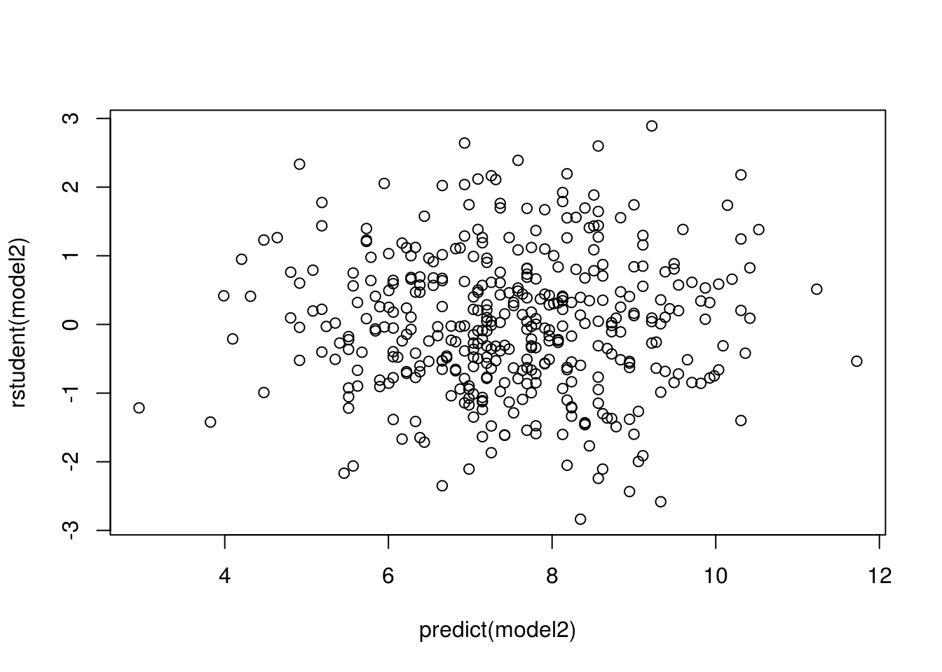
All studentized residuals appear to be bounded by -3 to 3, so no potential outliers are suggested from the linear regression.
par(mfrow=c(2,2))
plot(model2)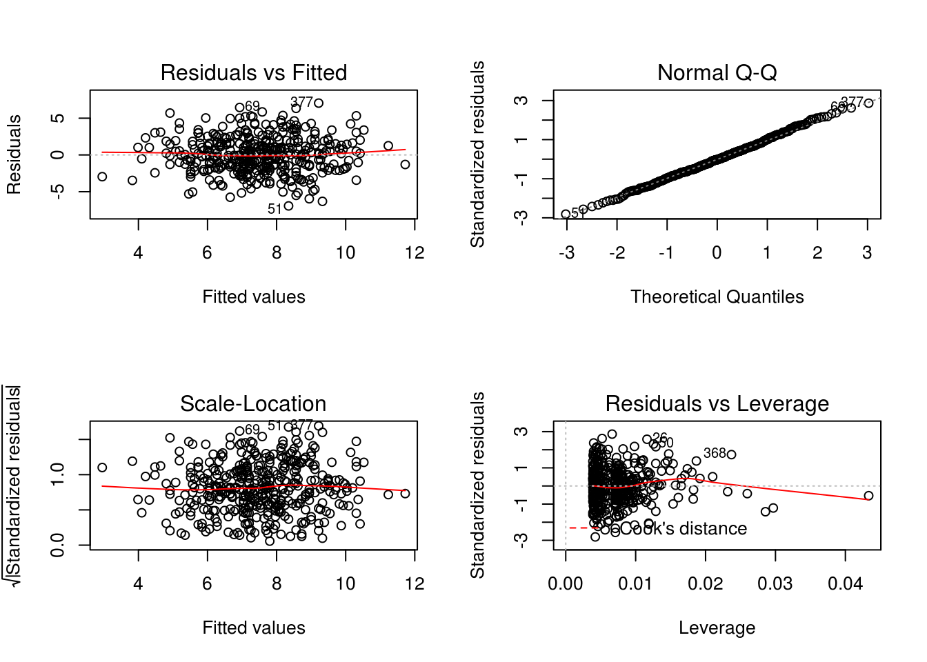
There are a few observations that greatly exceed \((p+1)/n\) (0.0075567) on the leverage-statistic plot that suggest that the corresponding points have high leverage.
2.2.3 Exercise
In this exercise you will create some simulated data and will fit simple linear regression models to it. Make sure to use set.seed() prior to starting part (a) to ensure consistent results.
- Using the
rnorm()function, create a vector,x, containing 100 observations drawn from a \(N(0,1)\) distribution. This represents a feature,X.
set.seed(12345)
x <- rnorm(100)- Using the
rnorm()function, create a vector,eps, containing 100 observations drawn from a \(N(0,0.25)\) distribution i.e. a normal distribution with mean zero and variance 0.25.
eps <- rnorm(100, 0, sqrt(0.25))- Using
xandeps, generate a vectoryaccording to the model \[Y = -1 + 0.5X + \epsilon\] What is the length of the vectory? What are the values of \(\beta_0\) and \(\beta_1\) in this linear model?
y = -1 + 0.5*x + epsy is of length 100. \(\beta_0\) is -1, \(\beta_1\) is 0.5.
- Create a scatterplot displaying the relationship between
xandy. Comment on what you observe.
plot(x, y)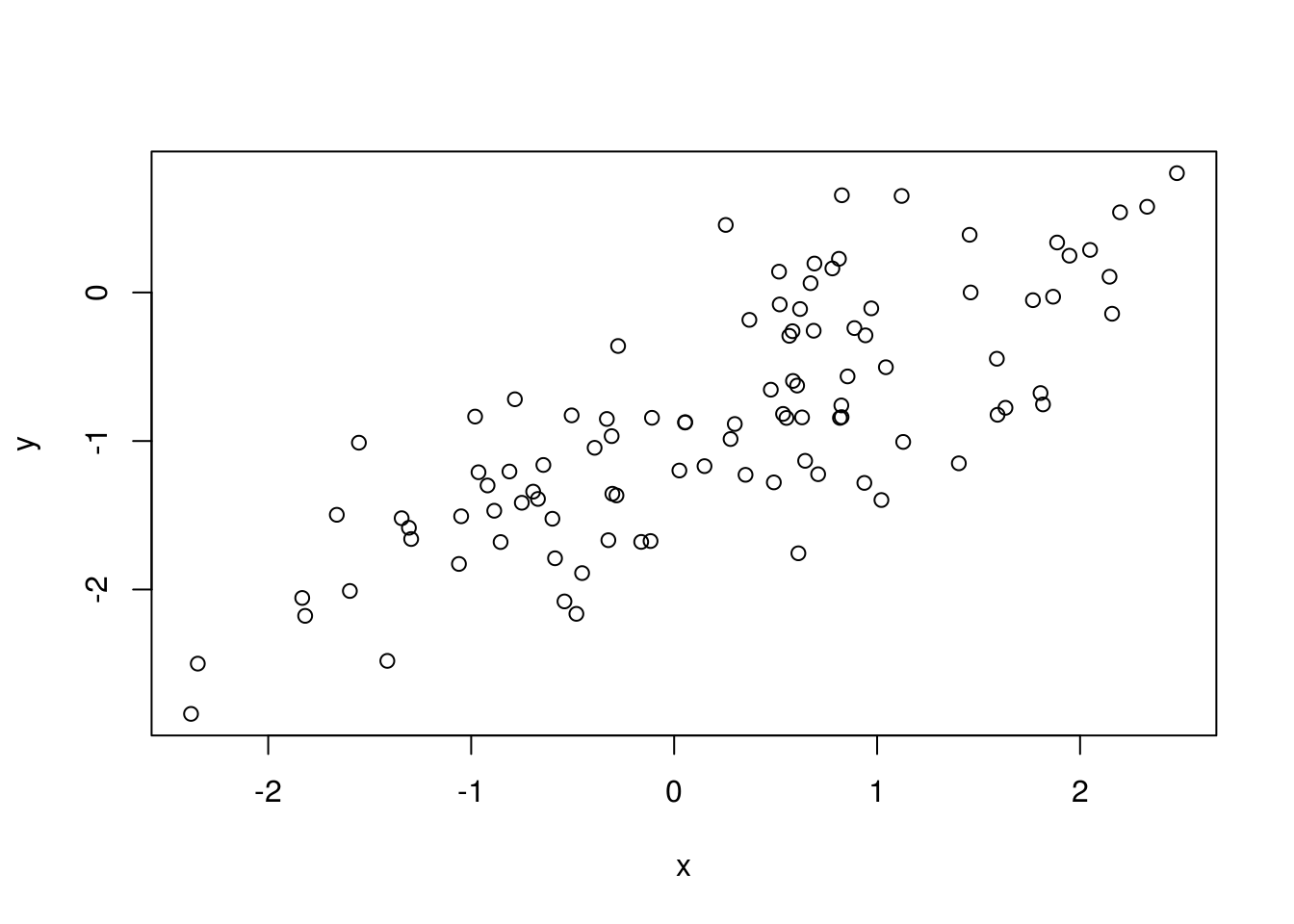
A linear relationship between x and y with a positive slope, with a variance as is to be expected.
- Fit a least squares linear model to predict
yusingx. Comment on the model obtained. How do \(\hat{\beta}_0\) and \(\hat{\beta}_1\) compare to \(\beta_0\) and \(\beta_1\)?
model1 <- lm(y ~ x)
summary(model1)
Call:
lm(formula = y ~ x)

Residuals:
     Min       1Q   Median       3Q      Max
-1.10174 -0.30139 -0.00557  0.30949  1.30485

Coefficients:
            Estimate Std. Error t value Pr(>|t|)
(Intercept) -0.98897    0.05176  -19.11   <2e-16 ***
x            0.54727    0.04557   12.01   <2e-16 ***
---
Signif. codes:  0 '***' 0.001 '**' 0.01 '*' 0.05 '.' 0.1 ' ' 1

Residual standard error: 0.5054 on 98 degrees of freedom
Multiple R-squared:  0.5954,    Adjusted R-squared:  0.5913
F-statistic: 144.2 on 1 and 98 DF,  p-value: < 2.2e-16
The linear regression fits a model close to the true value of the coefficients as was constructed. The model has a large F-statistic with a near-zero p-value so the null hypothesis can be rejected.
- Display the least squares line on the scatterplot obtained in (d). Draw the population regression line on the plot, in a different color. Use the
legend()command to create an appropriate legend.
plot(x, y)
abline(model1, col = "blue")
abline(-1, 0.5, col = "red")
legend(-1, legend = c("model fit", "pop. regression"), col=c("blue", "red"), lwd=1)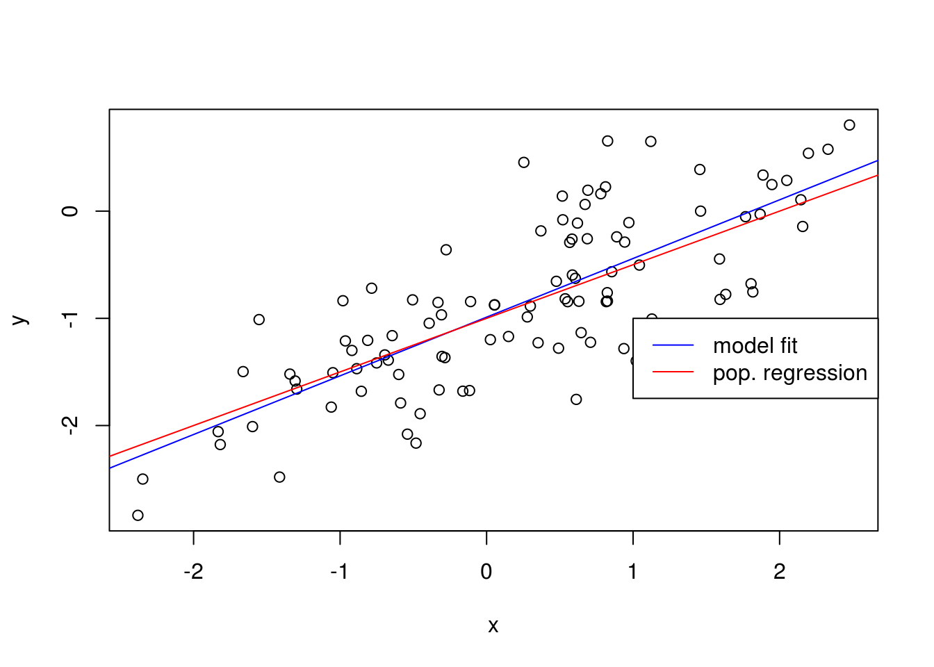
- Now fit a polynomial regression model that predicts \(y\) using \(x\) and \(x^2\). Is there evidence that the quadratic term improves the model fit? Explain your answer.
model_poly <-  lm(y ~ x + I(x^2))
summary(model_poly)
Call:
lm(formula = y ~ x + I(x^2))

Residuals:
     Min       1Q   Median       3Q      Max
-1.12465 -0.29431  0.00067  0.33213  1.27769

Coefficients:
            Estimate Std. Error t value Pr(>|t|)
(Intercept) -0.96224    0.06669 -14.429   <2e-16 ***
x            0.55456    0.04711  11.771   <2e-16 ***
I(x^2)      -0.02210    0.03461  -0.639    0.525
---
Signif. codes:  0 '***' 0.001 '**' 0.01 '*' 0.05 '.' 0.1 ' ' 1

Residual standard error: 0.507 on 97 degrees of freedom
Multiple R-squared:  0.5971,    Adjusted R-squared:  0.5888
F-statistic: 71.88 on 2 and 97 DF,  p-value: < 2.2e-16
There is evidence that model fit has increased over the training data given the slight increase in \(R^2\). Although, the p-value of the t-statistic suggests that there isn’t a relationship between y and \(x^2\).
- Repeat (a)-(f) after modifying the data generation process in such a way that there is less noise in the data. The model should remain the same. You can do this by decreasing the variance of the normal distribution used to generate the error term \(\epsilon\) in (b). Describe your results.
set.seed(12345)
eps <- rnorm(100, 0, 0.125)
x <- rnorm(100)
y <-  -1 + 0.5*x + eps
plot(x, y)
model2 <- lm(y ~ x)
summary(model2)
Call:
lm(formula = y ~ x)

Residuals:
     Min       1Q   Median       3Q      Max
-0.31403 -0.10026  0.02081  0.07945  0.26341

Coefficients:
            Estimate Std. Error t value Pr(>|t|)
(Intercept) -0.97000    0.01394  -69.57   <2e-16 ***
x            0.51436    0.01384   37.16   <2e-16 ***
---
Signif. codes:  0 '***' 0.001 '**' 0.01 '*' 0.05 '.' 0.1 ' ' 1

Residual standard error: 0.1393 on 98 degrees of freedom
Multiple R-squared:  0.9337,    Adjusted R-squared:  0.933
F-statistic: 1381 on 1 and 98 DF, p-value: < 2.2e-16abline(model2, col = "blue")
abline(-1, 0.5, col = "red")
legend(-1, legend = c("model fit", "pop. regression"), col=c("blue", "red"), lwd=1)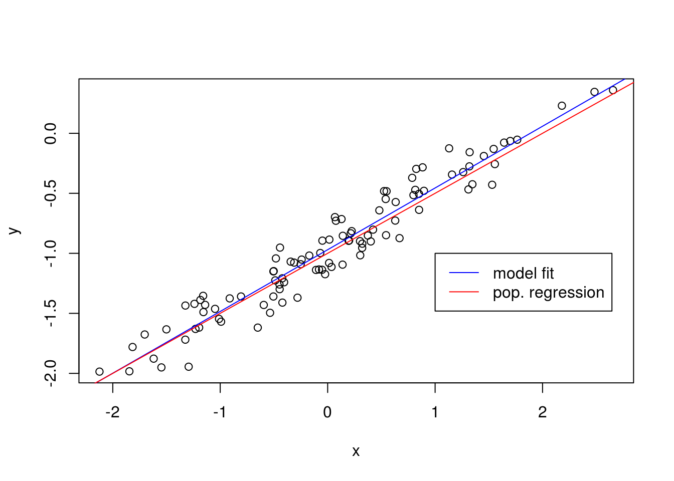
As expected, the error observed in the values of \(R^2\) decreases considerably.
- Repeat (a)-(f) after modifying the data generation process in such a way that there is more noise in the data. The model should remain the same. You can do this by increasing the variance of the normal distribution used to generate the error term \(\epsilon\) in (b). Describe your results.
set.seed(12345)
eps <- rnorm(100, 0, 0.5)
x <- rnorm(100)
y <-  -1 + 0.5*x + eps
plot(x, y)
model3 <- lm(y ~ x)
summary(model3)
Call:
lm(formula = y ~ x)

Residuals:
     Min       1Q   Median       3Q      Max
-1.25611 -0.40103  0.08324  0.31779  1.05363

Coefficients:
            Estimate Std. Error t value Pr(>|t|)
(Intercept) -0.88000    0.05577  -15.78   <2e-16 ***
x            0.55744    0.05537   10.07   <2e-16 ***
---
Signif. codes:  0 '***' 0.001 '**' 0.01 '*' 0.05 '.' 0.1 ' ' 1

Residual standard error: 0.5572 on 98 degrees of freedom
Multiple R-squared:  0.5084,    Adjusted R-squared:  0.5034
F-statistic: 101.3 on 1 and 98 DF, p-value: < 2.2e-16abline(model3, col = "blue")
abline(-1, 0.5, col = "red")
legend(-1, legend = c("model fit", "pop. regression"), col=c("blue", "red"), lwd=1)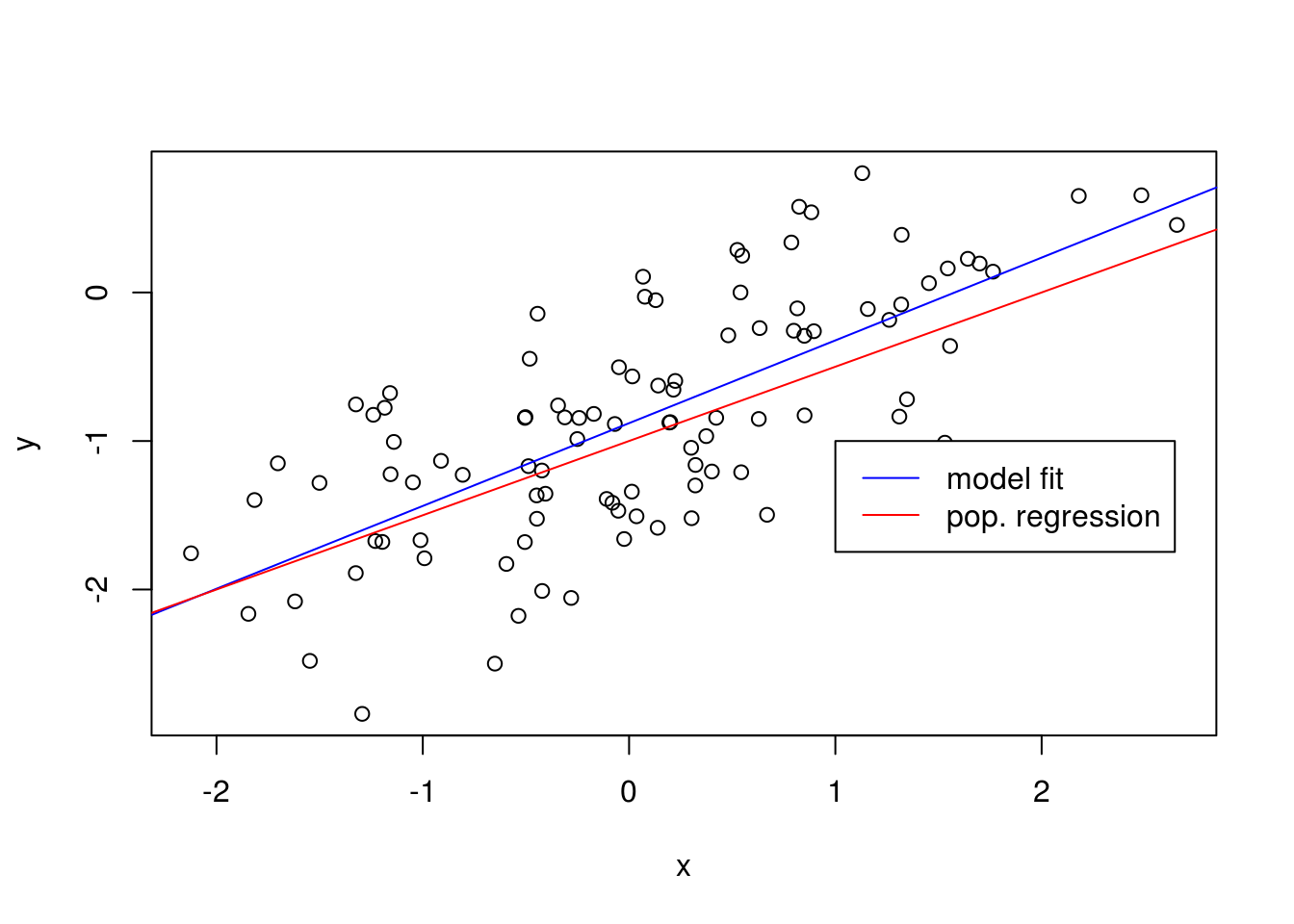
As expected, the error observed in \(R^2\) and \(RSE\) increases considerably.
- What are the confidence intervals for \(\beta_0\) and \(\beta_1\) based on the original data set, the noisier data set, and the less noisy data set? Comment on your results.
confint(model1) 2.5 % 97.5 %
(Intercept) -1.0916952 -0.8862514
x 0.4568371 0.6376979confint(model2) 2.5 % 97.5 %
(Intercept) -0.9976690 -0.9423307
x 0.4868876 0.5418310confint(model3) 2.5 % 97.5 %
(Intercept) -0.9906761 -0.7693228
x 0.4475505 0.6673240All intervals seem to be centered on approximately 0.5, with the second fit’s interval being narrower than the first fit’s interval and the last fit’s interval being wider than the first fit’s interval.
2.2.4 Optional Exercise
- Install the
regsimpackage.
Follow the instructions on regsim documentation page to install the package. If you don’t already have devtools package installed, then install that first.
- For any of the linear models estimated in previous exercises, use
regsimto run simulations and plot confidence interval plots.
Let’s try regsim with the last two models we estimated.
library(regsim)

sim <- regsim(model2, list(x = x))
plot(sim)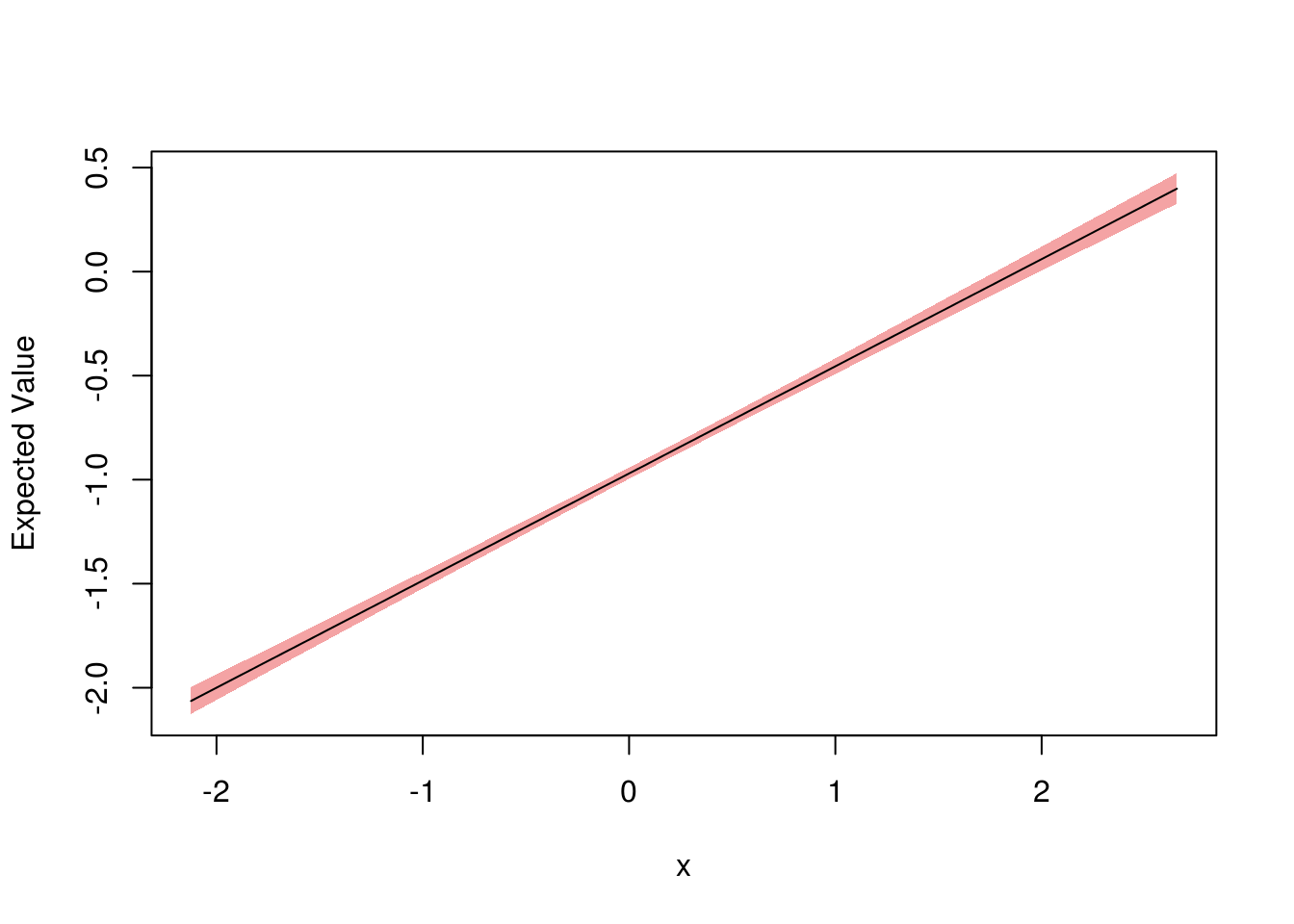
sim <- regsim(model3, list(x = x))
plot(sim)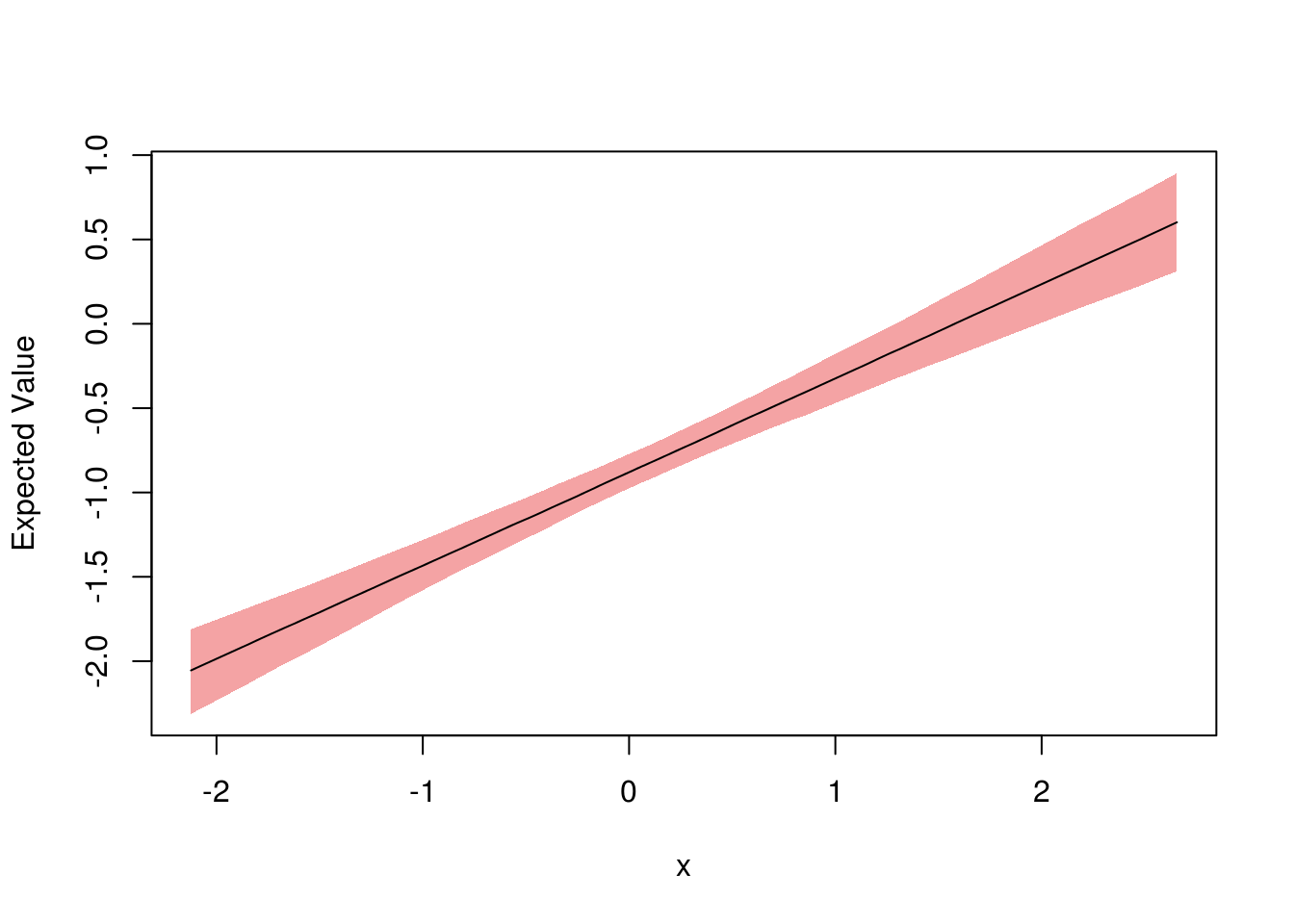
Now let’s try regsim with multiple regression using Carseats dataset.
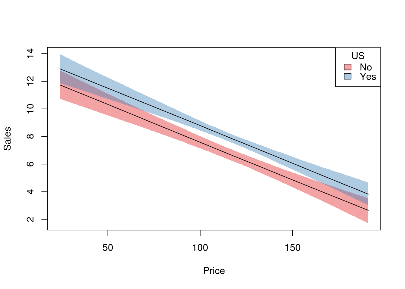
model <- lm(Sales ~ Price + US, data = Carseats)

xprofiles <- list(
  Price = seq(min(Carseats$Price), max(Carseats$Price), length=100),
  US = levels(Carseats$US)
)
sim <- regsim(model, xprofiles)

plot(sim, ylab = "Sales")