5.2 Solutions
5.2.1 Exercise
This question relates to the College dataset from the ISLR package.
- Split the data into a training set and a test set. Using out-of-state tuition as the response and the other variables as the predictors, perform forward stepwise selection on the training set in order to identify a satisfactory model that uses just a subset of the predictors.
library(ISLR)
library(leaps)
library(gam)
library(gbm)
library(glmnet)
library(randomForest)set.seed(12345)
train <- sample(nrow(College) * 0.7)
train_set <- College[train, ]
test_set <- College[-train, ]forward_subset <- regsubsets(Outstate ~ ., data = train_set, nvmax = ncol(College)-1, method = "forward")
model_summary <- summary(forward_subset)
plot_metric <- function(metric, yaxis_label, reverse = FALSE) {
plot(metric, xlab = "Number of Variables", ylab = yaxis_label, xaxt = "n", type = "l")
axis(side = 1, at = 1:length(metric))
if (reverse) {
metric_1se <- max(metric) - (sd(metric) / sqrt(length(metric)))
min_subset <- which(metric > metric_1se)
} else {
metric_1se <- min(metric) + (sd(metric) / sqrt(length(metric)))
min_subset <- which(metric < metric_1se)
}
abline(h = metric_1se, col = "red", lty = 2)
abline(v = min_subset[1], col = "green", lty = 2)
}
par(mfrow=c(1, 3))
plot_metric(model_summary$cp, "Cp")
plot_metric(model_summary$bic, "BIC")
plot_metric(model_summary$adjr2, "Adjusted R2", reverse = TRUE) # higher values are better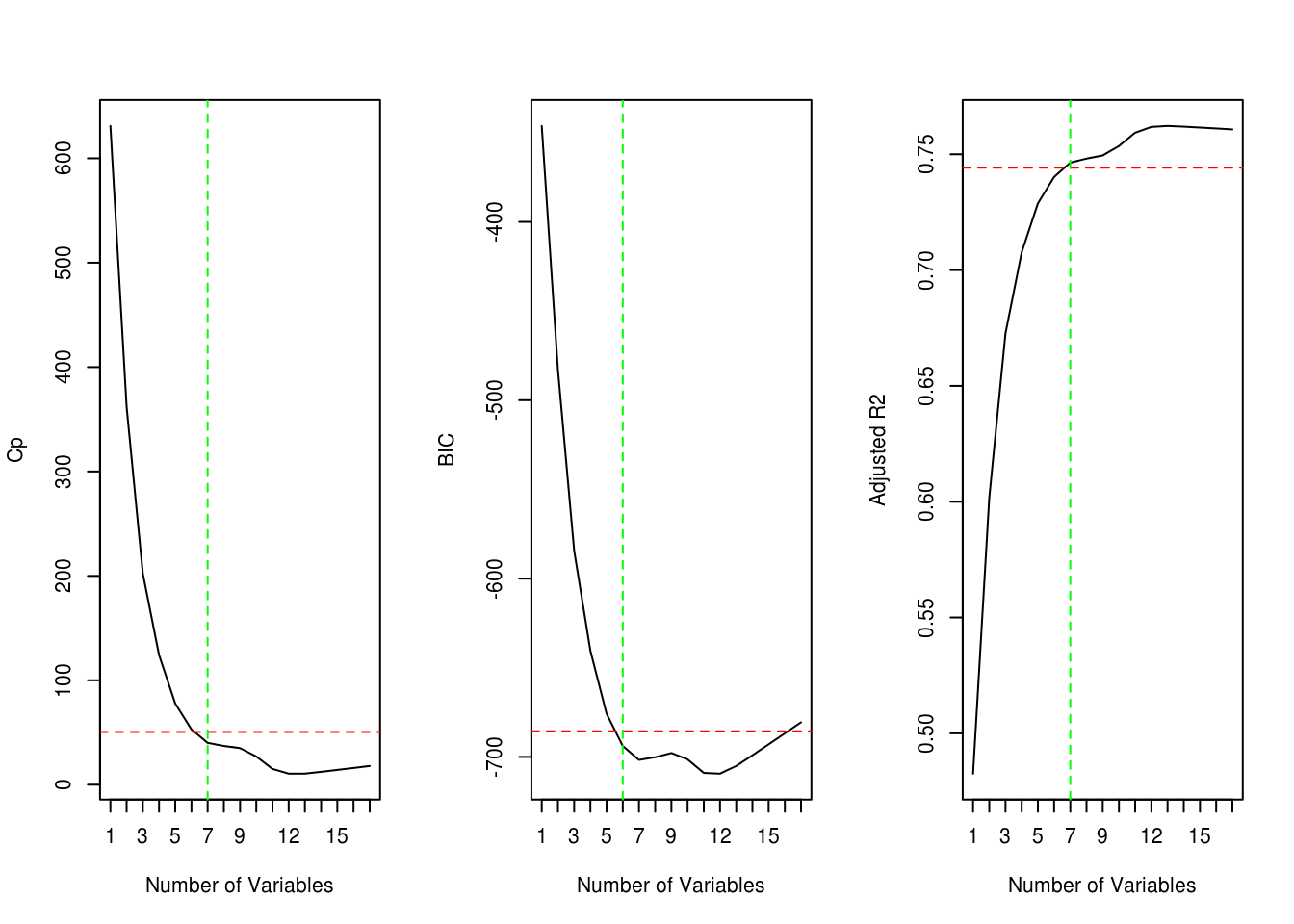
The red dotted line shows the best metric (Cp, BIC, Adjusted R2) within 1 standard error. The green dotted line shows the subset for best metric with the smallest number of variables. Cp and Adjusted R2 give us a subset with 7 variables and BIC gives us 6.
coef(forward_subset, 6) (Intercept) PrivateYes Room.Board PhD perc.alumni
-3769.0587788 2748.6944010 0.8999634 38.5143460 44.4889713
Expend Grad.Rate
0.2543900 31.2043096 - Fit a GAM on the training data, using out-of-state tuition as the response and the features selected in the previous step as the predictors. Plot the results, and explain your findings.
gam_model <- gam(Outstate ~ Private + s(Room.Board, df=2) + s(perc.alumni, df=2) +
                   s(PhD, df=2) + s(Expend, df=2) + s(Grad.Rate, df=2), data=train_set)
par(mfrow=c(2, 3))
plot(gam_model, se=TRUE, col="blue")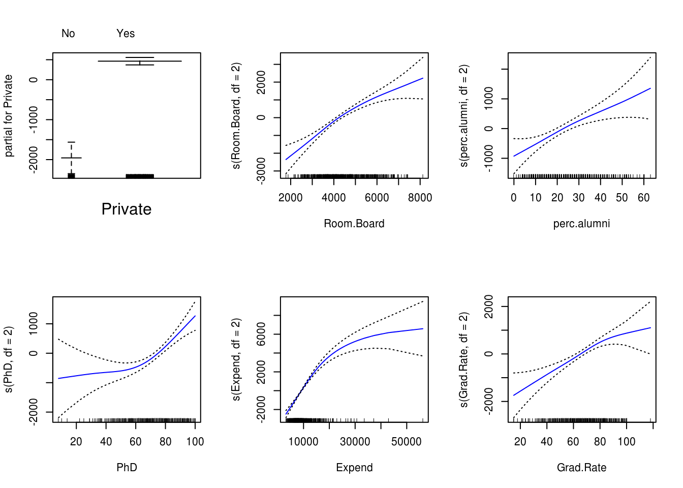
- Evaluate the model obtained on the test set, and explain the results obtained.
Re-use some functions for calculating RMSE and R^2 from last week:
calc_mse <- function(y, y_hat) {
  return(mean((y - y_hat)^2))
}

calc_rmse <- function(y, y_hat) {
  return(sqrt(calc_mse(y, y_hat)))
}

calc_r2 <- function(y, y_hat) {
  y_bar <- mean(y)
  rss <- sum((y - y_hat)^2)
  tss <- sum((y - y_bar)^2)
  return(1 - (rss / tss))
}
gam_predictions <- predict(gam_model, test_set)
gam_rmse <- calc_rmse(test_set$Outstate, gam_predictions)
cat("RMSE:", gam_rmse, "\n")RMSE: 1984.385 gam_r2 <- calc_r2(test_set$Outstate, gam_predictions)
cat(" R^2:", gam_r2, "\n") R^2: 0.7614328 We obtain a test RMSE of 1984.3845506 and R-squared of 0.7614328 using GAM with 6 predictors
- For which variables, if any, is there evidence of a non-linear relationship with the response?
summary(gam_model)
Call: gam(formula = Outstate ~ Private + s(Room.Board, df = 2) + s(perc.alumni,
    df = 2) + s(PhD, df = 2) + s(Expend, df = 2) + s(Grad.Rate,
    df = 2), data = train_set)
Deviance Residuals:
      Min        1Q    Median        3Q       Max
-7164.185 -1192.389     9.746  1195.918  8668.434

(Dispersion Parameter for gaussian family taken to be 3515849)

    Null Deviance: 8614032615 on 542 degrees of freedom
Residual Deviance: 1866916246 on 531.0002 degrees of freedom
AIC: 9739.358

Number of Local Scoring Iterations: 2

Anova for Parametric Effects
                        Df     Sum Sq    Mean Sq F value    Pr(>F)
Private                  1 1968096326 1968096326 559.778 < 2.2e-16 ***
s(Room.Board, df = 2)    1 1852547004 1852547004 526.913 < 2.2e-16 ***
s(perc.alumni, df = 2)   1  739433651  739433651 210.314 < 2.2e-16 ***
s(PhD, df = 2)           1  408910513  408910513 116.305 < 2.2e-16 ***
s(Expend, df = 2)        1  669471699  669471699 190.415 < 2.2e-16 ***
s(Grad.Rate, df = 2)     1  105813593  105813593  30.096 6.372e-08 ***
Residuals              531 1866916246    3515849
---
Signif. codes:  0 '***' 0.001 '**' 0.01 '*' 0.05 '.' 0.1 ' ' 1

Anova for Nonparametric Effects
                       Npar Df Npar F     Pr(F)
(Intercept)
Private
s(Room.Board, df = 2)        1  5.624 0.0180708 *
s(perc.alumni, df = 2)       1  0.517 0.4725226
s(PhD, df = 2)               1 11.780 0.0006455 ***
s(Expend, df = 2)            1 70.804 4.441e-16 ***
s(Grad.Rate, df = 2)         1  3.159 0.0761031 .
---
Signif. codes:  0 '***' 0.001 '**' 0.01 '*' 0.05 '.' 0.1 ' ' 1
Non-parametric Anova test shows a strong evidence of non-linear relationship between response and Expend and PhD, and a moderately strong non-linear relationship between response and Room.Board and Grad.Rate.
5.2.2 Exercise
Apply boosting, bagging, and random forests to a data set of your choice. Be sure to fit the models on a training set and to evaluate their performance on a test set. How accurate are the results compared to simple methods like linear or logistic regression? Which of these approaches yields the best performance?
data(Weekly)
Weekly$Direction <- Weekly$Direction == "Up"
Weekly <- subset(Weekly, select = -c(Year, Today)) # drop Year and Today columns

set.seed(12345)
train <- sample(nrow(Weekly) * 0.7)
train_set <- Weekly[train, ]
test_set <- Weekly[-train, ]
# show confusion matrix from predicted class and observed class
show_model_performance <- function(predicted_status, observed_status) {
confusion_matrix <- table(predicted_status,
observed_status,
dnn = c("Predicted Status", "Observed Status"))
print(confusion_matrix)
error_rate <- mean(predicted_status != observed_status)
cat("\n") # \n means newline so it just prints a blank line
cat(" Error Rate:", 100 * error_rate, "%\n")
cat("Correctly Predicted:", 100 * (1-error_rate), "%\n")
cat("False Positive Rate:", 100 * confusion_matrix[2,1] / sum(confusion_matrix[,1]), "%\n")
cat("False Negative Rate:", 100 * confusion_matrix[1,2] / sum(confusion_matrix[,2]), "%\n")
}Logistic regression
logit_model <- glm(Direction ~ ., data = Weekly, family = binomial, subset = train)

predicted_direction <- predict(logit_model, test_set, type="response") > 0.5
show_model_performance(predicted_direction, test_set$Direction)
Observed Status
Predicted Status FALSE TRUE
FALSE 128 157
TRUE 18 24
Error Rate: 53.51682 %
Correctly Predicted: 46.48318 %
False Positive Rate: 12.32877 %
False Negative Rate: 86.74033 %Boosting
boost_model <- gbm(Direction ~ ., data = train_set, n.trees=5000, distribution = "bernoulli")

predicted_direction <- predict(boost_model, test_set, n.trees=5000) > 0.5
show_model_performance(predicted_direction, test_set$Direction)
Observed Status
Predicted Status FALSE TRUE
FALSE 116 143
TRUE 30 38
Error Rate: 52.9052 %
Correctly Predicted: 47.0948 %
False Positive Rate: 20.54795 %
False Negative Rate: 79.00552 %Bagging
Weekly$Direction <- as.factor(Weekly$Direction)
bag_model <- randomForest(Direction ~ ., data=Weekly, subset=train, mtry=ncol(Weekly)-1)

predicted_direction <- predict(bag_model, test_set)
show_model_performance(predicted_direction, test_set$Direction)
Observed Status
Predicted Status FALSE TRUE
FALSE 18 23
TRUE 128 158
Error Rate: 46.17737 %
Correctly Predicted: 53.82263 %
False Positive Rate: 87.67123 %
False Negative Rate: 12.70718 %Random Forests
rf_model <- randomForest(Direction ~ ., data=Weekly, subset=train, mtry=2)

predicted_direction <- predict(rf_model, test_set)
show_model_performance(predicted_direction, test_set$Direction)
Observed Status
Predicted Status FALSE TRUE
FALSE 21 25
TRUE 125 156
Error Rate: 45.87156 %
Correctly Predicted: 54.12844 %
False Positive Rate: 85.61644 %
False Negative Rate: 13.81215 %5.2.3 Exercise
We now use boosting to predict Salary in the Hitters dataset, which is part of the ISLR package.
- Remove the observations for whom the salary information is unknown, and then log-transform the salaries.
sum(is.na(Hitters$Salary))[1] 59Hitters <- Hitters[-which(is.na(Hitters$Salary)), ]
sum(is.na(Hitters$Salary))[1] 0Hitters$Salary <- log(Hitters$Salary)- Create a training set consisting of the first 200 observations, and a test set consisting of the remaining observations.
train <- 1:200
train_set <- Hitters[train, ]
test_set <- Hitters[-train, ]- Perform boosting on the training set with 1,000 trees for a range of values of the shrinkage parameter \(\lambda\). Produce a plot with different shrinkage values on the \(x\)-axis and the corresponding training set MSE on the \(y\)-axis.
set.seed(12345)
lambdas <- 10 ^ seq(-10, -0.2, length = 100)
train_errors <- rep(NA, length(lambdas))
test_errors <- rep(NA, length(lambdas))

for (i in 1:length(lambdas)) {
  boost_model <- gbm(Salary ~ . , data = train_set, distribution = "gaussian",
                       n.trees = 1000, shrinkage = lambdas[i])

  train_predictions <- predict(boost_model, train_set, n.trees = 1000)
  train_errors[i] <- calc_mse(train_set$Salary, train_predictions)

  test_predictions <- predict(boost_model, test_set, n.trees = 1000)
  test_errors[i] <- calc_mse(test_set$Salary, test_predictions)
}

plot(lambdas, train_errors, xlab = "Shrinkage", ylab = "Train MSE", col = "blue", type = "b", pch = 20)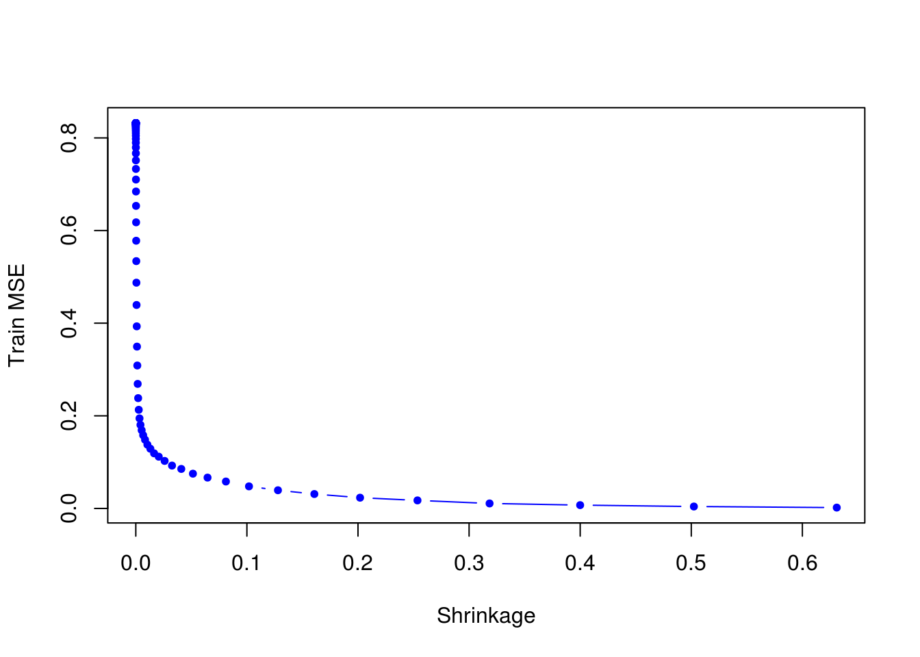
- Produce a plot with different shrinkage values on the \(x\)-axis and the corresponding test set MSE on the \(y\)-axis.
plot(lambdas, test_errors, xlab = "Shrinkage", ylab = "Test MSE", col = "red", type = "b", pch = 20)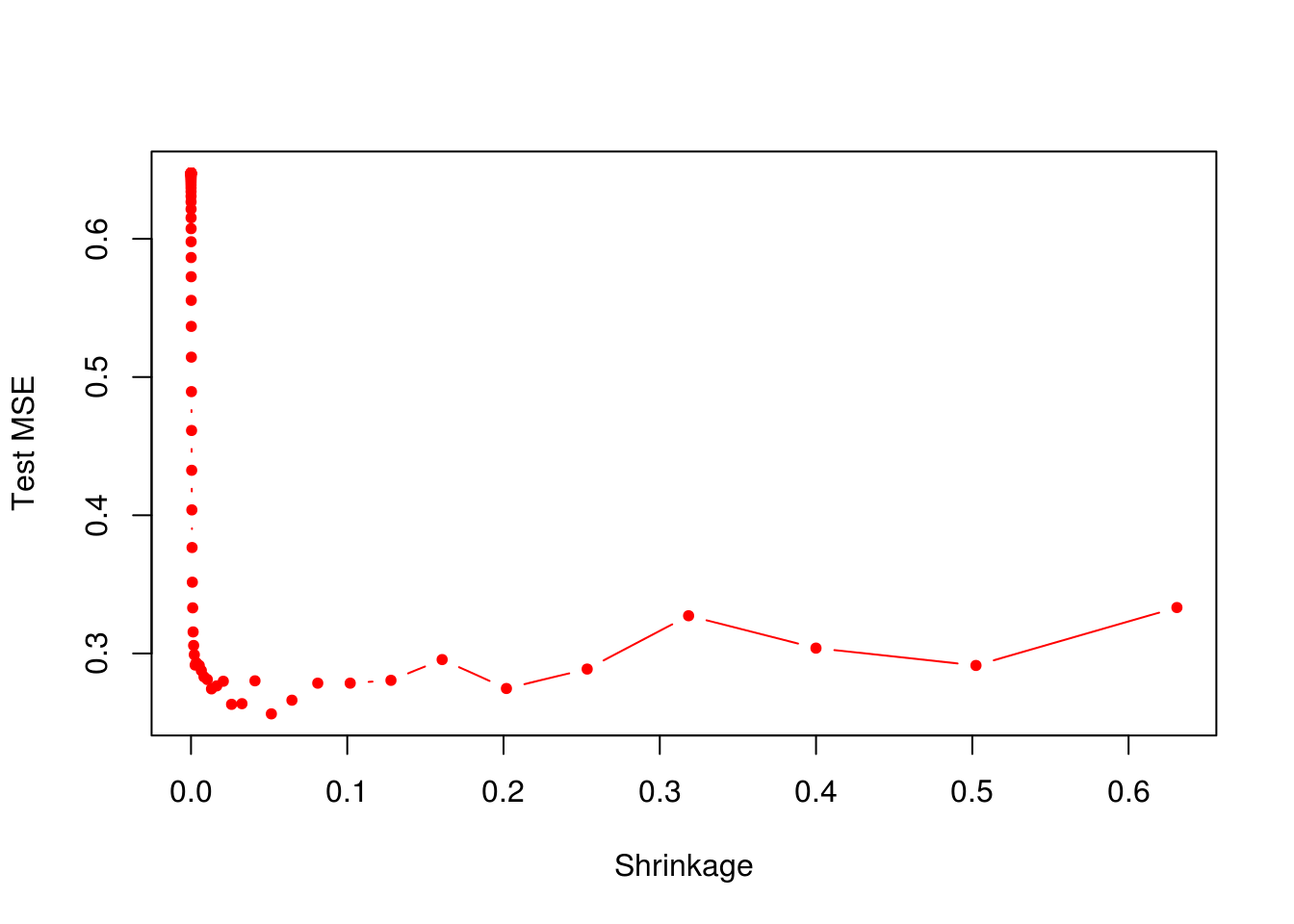
min(test_errors)[1] 0.256307boost_lambda_min <- lambdas[which.min(test_errors)]
boost_lambda_min[1] 0.05141752Minimum test error is obtained at \(\lambda = 0.0514175\).
- Compare the test MSE of boosting to the test MSE that results from applying two of the regression approaches seen in our discussions of regression models.
OLS
ols_model <- lm(Salary ~ . , data = train_set)
ols_predictions <- predict(ols_model, test_set)
calc_mse(test_set$Salary, ols_predictions)
[1] 0.4917959Lasso
set.seed(12345)

train_matrix <- model.matrix(Salary ~ . , data = train_set)
test_matrix <- model.matrix(Salary ~ . , data = test_set)

lasso_model <- glmnet(train_matrix, train_set$Salary, alpha = 1)
lasso_predictions <- predict(lasso_model, s=0.01, newx=test_matrix)

calc_mse(test_set$Salary, lasso_predictions)
[1] 0.4700537Both linear model and regularization like Lasso have higher test MSE than boosting.
- Which variables appear to be the most important predictors in the boosted model?
boost_model <- gbm(Salary ~ . , data = train_set, distribution="gaussian",
                   n.trees = 1000, shrinkage = boost_lambda_min)
summary(boost_model)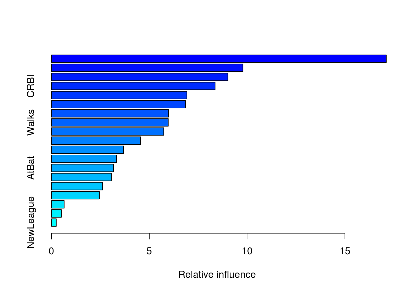
                var    rel.inf
CAtBat       CAtBat 17.1188801
CHits         CHits  9.7853653
CWalks       CWalks  9.0182320
CRBI           CRBI  8.3641950
Years         Years  6.9200672
PutOuts     PutOuts  6.8526315
CRuns         CRuns  5.9824324
Walks         Walks  5.9709905
CHmRun       CHmRun  5.7374204
Hits           Hits  4.5490252
RBI             RBI  3.6855364
Assists     Assists  3.3276611
AtBat         AtBat  3.1707344
HmRun         HmRun  3.0619600
Errors       Errors  2.6103787
Runs           Runs  2.4470517
Division   Division  0.6477526
League       League  0.5066292
NewLeague NewLeague 0.2430562CAtBat, CHits and CWalks are three most important variables in that order.
- Now apply bagging to the training set. What is the test set MSE for this approach?
set.seed(12345)
rf_model <- randomForest(Salary ~ . , data = train_set, ntree = 500, mtry = ncol(train_set)-1)
rf_predictions <- predict(rf_model, test_set)

rf_mse <- calc_mse(test_set$Salary, rf_predictions)
rf_mse
[1] 0.2291436Test MSE for bagging is about \(0.2291436\), which is slightly lower than the best test MSE for boosting.