Structural Topic Models
For more information on Structural Topic Models, take a look at http://www.structuraltopicmodel.com and also check out Brandon Stewart’s Dataverse where he shares his R code and datasets for a number of projects.
library(quanteda)
library(readtext)
library(stm)
Load the dataset from the CMU 2008 Political Blog Corpus. It contains blogs written about American politics during the 2008 election campaign.
blogs <- readtext("https://uclspp.github.io/datasets/data/poliblogs2008.zip")Create a corpus object using quanteda.
blogs_corpus <- corpus(blogs$documents, docvars = blogs)Create a document-feature matrix and trim the features.
blogs_dfm <- dfm(blogs_corpus,
                 stem = TRUE,
                 remove = stopwords("english"),
                 remove_punct = TRUE,
                 remove_numbers = TRUE)

blogs_dfm <- dfm_trim(blogs_dfm, min_count = 10, min_docfreq = 5)
Create a STM compatible document-feature matrix using the convert function.
blogs_dfm_stm <- convert(blogs_dfm, to = "stm", docvars = docvars(blogs_corpus))Run structural topic model with blog rating (conservative or liberal) and the date as dependent variables for topic prevalence.
system.time(
  stm_object <- stm(documents = blogs_dfm_stm$documents,
                    vocab = blogs_dfm_stm$vocab,
                    data = blogs_dfm_stm$meta,
                    prevalence = ~rating + s(day),
                    K = 20,
                    seed = 12345)
)
Plot the top topics
plot(stm_object)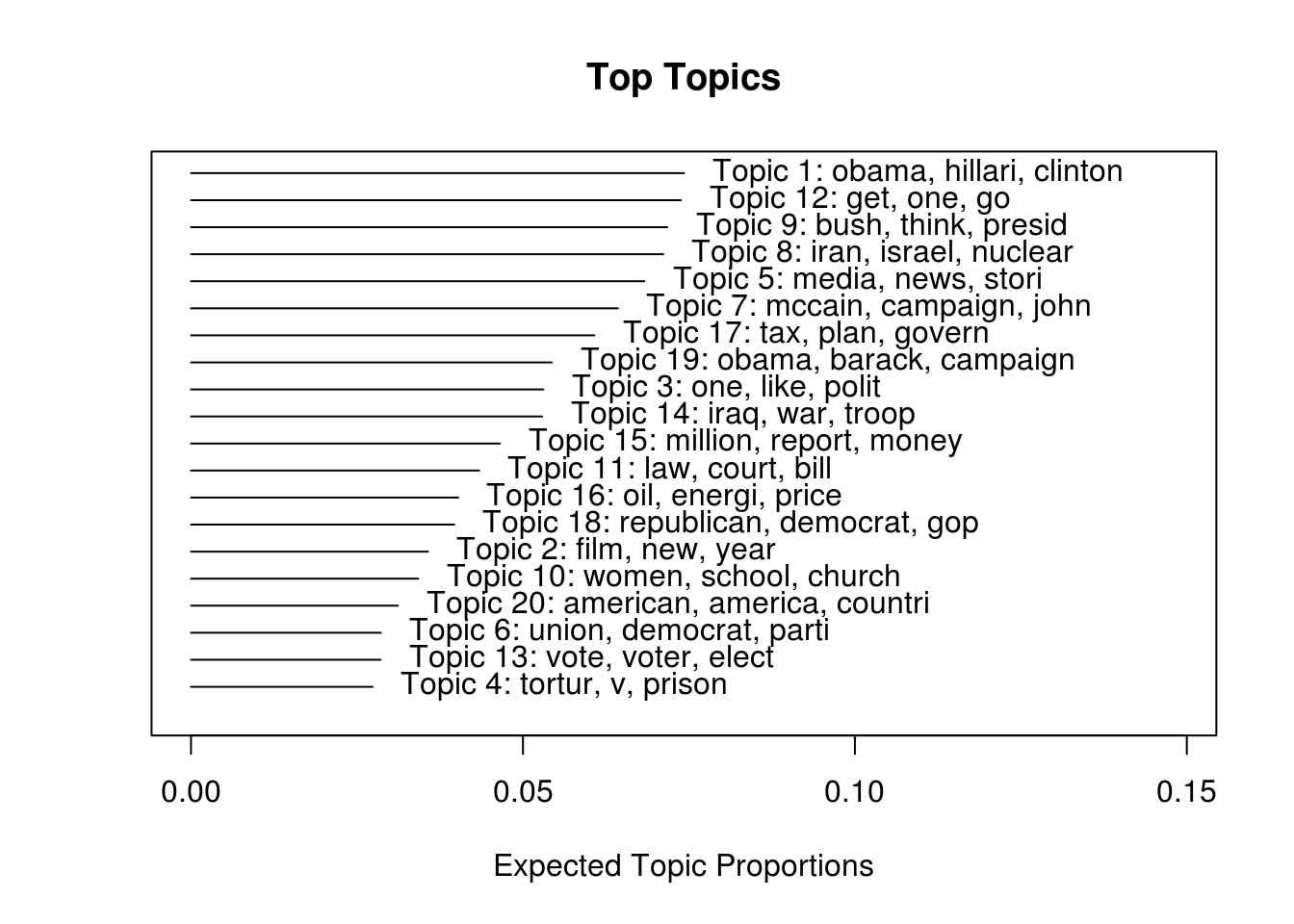
Pick the topics that are intersting to us and label them with something meaningful.
topics_of_interest <- c(5, 8, 14, 9)
topic_labels <- c("Media", "Iran", "Iraq", "Bush")
Estimate the effects of our predictors on the topics of interest.
stm_effects <- estimateEffect(topics_of_interest ~ rating + s(day),
                              stmobj = stm_object,
                              meta = blogs_dfm_stm$meta,
                              uncertainty = "Global")
Look at the regression output from the model
summary(stm_effects)
Call:
estimateEffect(formula = topics_of_interest ~ rating + s(day),
    stmobj = stm_object, metadata = blogs_dfm_stm$meta, uncertainty = "Global")


Topic 5:

Coefficients:
               Estimate Std. Error t value Pr(>|t|)
(Intercept)    0.065768   0.021404   3.073  0.00214 **
ratingLiberal -0.010833   0.004862  -2.228  0.02595 *
s(day)1       -0.010965   0.040989  -0.268  0.78908
s(day)2        0.005052   0.025709   0.197  0.84423
s(day)3        0.021345   0.028560   0.747  0.45489
s(day)4       -0.007256   0.025490  -0.285  0.77593
s(day)5        0.021745   0.027414   0.793  0.42770
s(day)6       -0.012530   0.024928  -0.503  0.61525
s(day)7        0.005613   0.028564   0.197  0.84423
s(day)8       -0.019137   0.030472  -0.628  0.53004
s(day)9        0.001449   0.034311   0.042  0.96632
s(day)10      -0.013038   0.030980  -0.421  0.67390
---
Signif. codes:  0 '***' 0.001 '**' 0.01 '*' 0.05 '.' 0.1 ' ' 1


Topic 8:

Coefficients:
               Estimate Std. Error t value Pr(>|t|)
(Intercept)    0.091987   0.030806   2.986  0.00285 **
ratingLiberal -0.064006   0.007001  -9.142  < 2e-16 ***
s(day)1       -0.028379   0.059007  -0.481  0.63058
s(day)2        0.043533   0.038948   1.118  0.26376
s(day)3        0.018182   0.041885   0.434  0.66425
s(day)4        0.056158   0.039140   1.435  0.15144
s(day)5       -0.010634   0.039135  -0.272  0.78584
s(day)6        0.010141   0.037284   0.272  0.78565
s(day)7       -0.071792   0.037008  -1.940  0.05248 .
s(day)8        0.046399   0.044685   1.038  0.29918
s(day)9       -0.073060   0.045276  -1.614  0.10670
s(day)10       0.072635   0.048892   1.486  0.13747
---
Signif. codes:  0 '***' 0.001 '**' 0.01 '*' 0.05 '.' 0.1 ' ' 1


Topic 14:

Coefficients:
               Estimate Std. Error t value Pr(>|t|)
(Intercept)    0.062572   0.026053   2.402  0.01637 *
ratingLiberal  0.015109   0.005698   2.652  0.00805 **
s(day)1       -0.043022   0.050119  -0.858  0.39073
s(day)2        0.033362   0.031561   1.057  0.29055
s(day)3        0.011962   0.034378   0.348  0.72790
s(day)4       -0.040140   0.033309  -1.205  0.22825
s(day)5        0.053431   0.032441   1.647  0.09965 .
s(day)6       -0.056598   0.030502  -1.856  0.06361 .
s(day)7       -0.042839   0.030694  -1.396  0.16290
s(day)8       -0.044735   0.035656  -1.255  0.20970
s(day)9       -0.004184   0.036877  -0.113  0.90967
s(day)10      -0.043006   0.038547  -1.116  0.26465
---
Signif. codes:  0 '***' 0.001 '**' 0.01 '*' 0.05 '.' 0.1 ' ' 1


Topic 9:

Coefficients:
                Estimate Std. Error t value Pr(>|t|)
(Intercept)    0.0319104  0.0215177   1.483    0.138
ratingLiberal  0.0822491  0.0051216  16.059   <2e-16 ***
s(day)1        0.0042269  0.0411741   0.103    0.918
s(day)2       -0.0004886  0.0257478  -0.019    0.985
s(day)3        0.0007390  0.0291158   0.025    0.980
s(day)4        0.0145598  0.0268477   0.542    0.588
s(day)5       -0.0062368  0.0249423  -0.250    0.803
s(day)6       -0.0095619  0.0277388  -0.345    0.730
s(day)7       -0.0074142  0.0243248  -0.305    0.761
s(day)8        0.0122285  0.0359506   0.340    0.734
s(day)9        0.0058710  0.0311423   0.189    0.850
s(day)10       0.0085972  0.0322449   0.267    0.790
---
Signif. codes:  0 '***' 0.001 '**' 0.01 '*' 0.05 '.' 0.1 ' ' 1
You can also show summary of individual topics if you prefer.
summary(stm_effects, topic = 8)
Call:
estimateEffect(formula = topics_of_interest ~ rating + s(day),
    stmobj = stm_object, metadata = blogs_dfm_stm$meta, uncertainty = "Global")


Topic 8:

Coefficients:
               Estimate Std. Error t value Pr(>|t|)
(Intercept)    0.065965   0.021672   3.044  0.00235 **
ratingLiberal -0.010837   0.004884  -2.219  0.02657 *
s(day)1       -0.011105   0.041648  -0.267  0.78977
s(day)2        0.005215   0.025853   0.202  0.84015
s(day)3        0.020788   0.028950   0.718  0.47278
s(day)4       -0.007155   0.025765  -0.278  0.78126
s(day)5        0.021350   0.027527   0.776  0.43804
s(day)6       -0.012451   0.025140  -0.495  0.62045
s(day)7        0.005198   0.028605   0.182  0.85582
s(day)8       -0.019116   0.030502  -0.627  0.53088
s(day)9        0.001184   0.034576   0.034  0.97269
s(day)10      -0.013319   0.031328  -0.425  0.67077
---
Signif. codes:  0 '***' 0.001 '**' 0.01 '*' 0.05 '.' 0.1 ' ' 1
Plot the marginal effects of blog rating (conservative vs. liberal) on topics. Conservative leaning blogs seem to discuss the media and Iran, while liberal leaning ones focus on Bush and Iraq.
plot(stm_effects,
     covariate = "rating",
     topics = topics_of_interest,
     model = stm_object,
     method = "difference",
     cov.value1 = "Liberal",
     cov.value2 = "Conservative",
     xlim = c(-0.1, 0.1),
     labeltype = "custom",
     custom.labels = topic_labels,
     main = "Effect of Liberal vs. Conservative",
     xlab = "More Conservative ... More Liberal")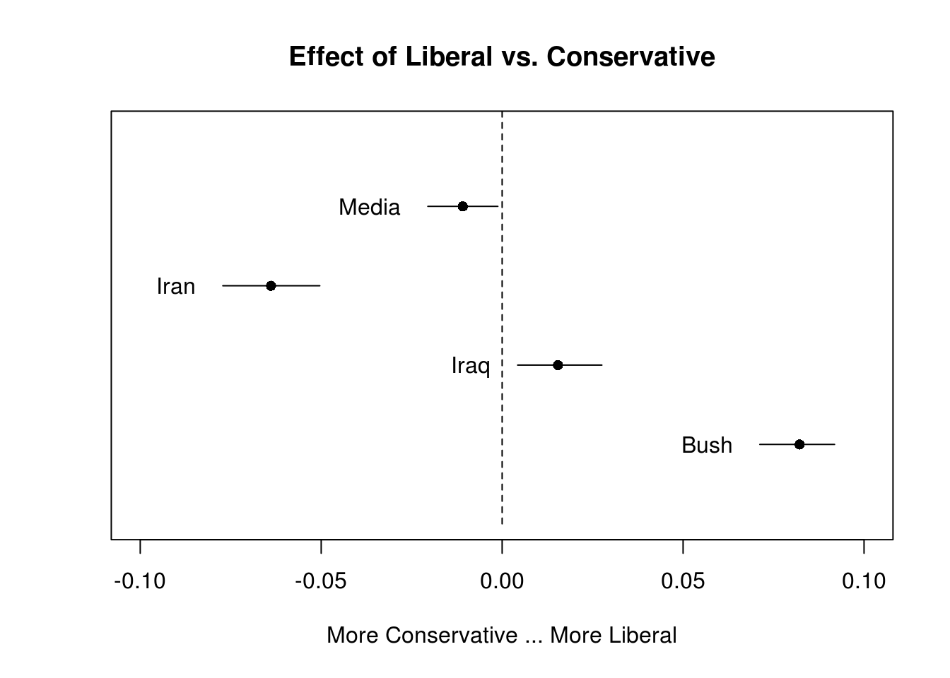
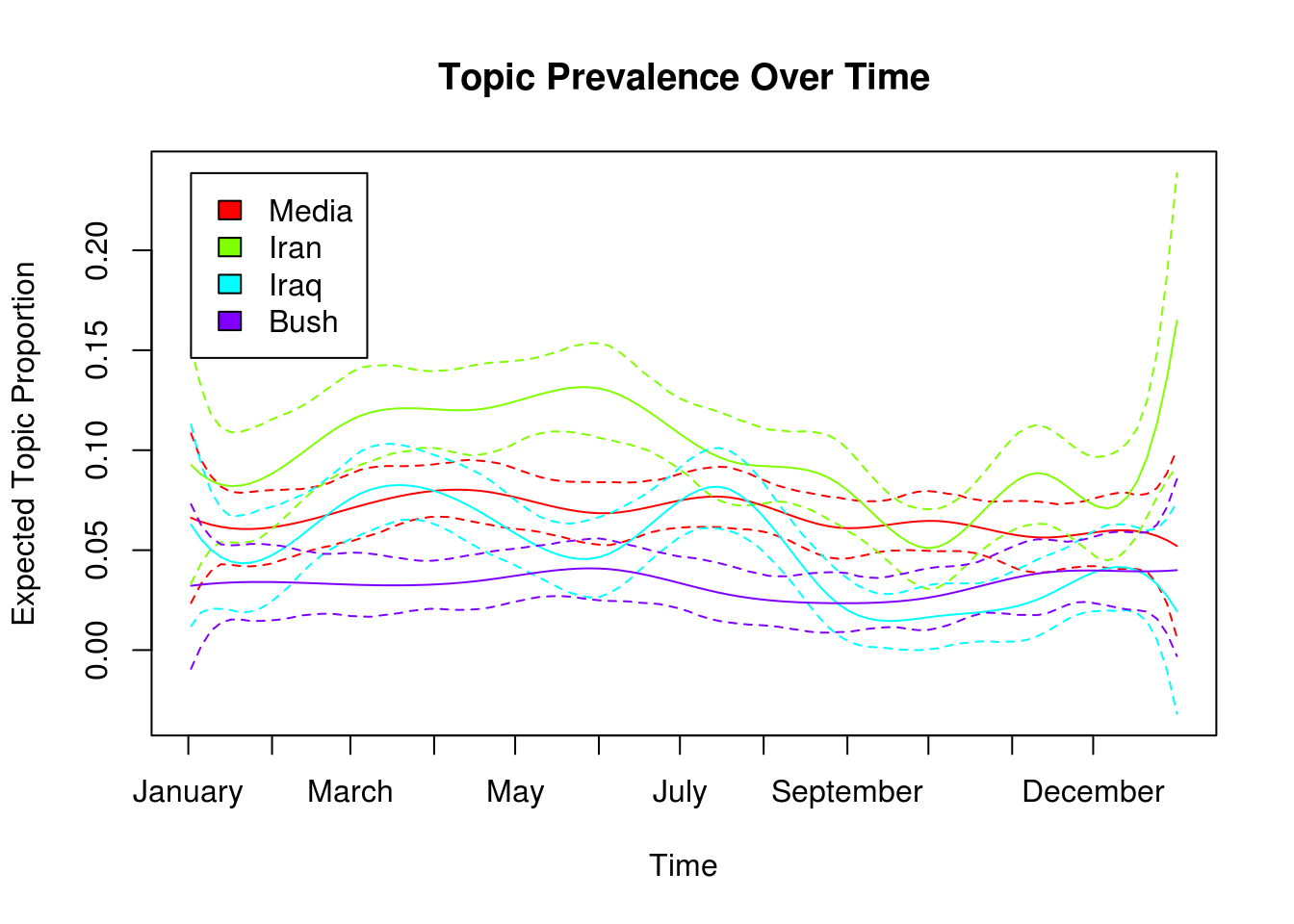
You can plot how the topic prevalence changes over time based on the date of the blog.
plot(stm_effects,
     covariate = "day",
     method = "continuous",
     topics = topics_of_interest,
     model = stm_object,
     labeltype = "custom",
     custom.labels = topic_labels,
     xaxt = "n",
     xlab = "Time",
     main = "Topic Prevalence Over Time"
)

# set the x-axis labels as month names
blog_dates <- seq(from = as.Date("2008-01-01"),
                  to = as.Date("2008-12-01"),
                  by = "month")

axis(1, blog_dates - min(blog_dates), labels = months(blog_dates))