3.2 Solutions
You will need to load the core library for the course textbook:
library(ISLR)3.2.1 Exercise
This question should be answered using the Weekly data set, which is part of the ISLR package. This data contains 1,089 weekly stock returns for 21 years, from the beginning of 1990 to the end of 2010.
- Produce some numerical and graphical summaries of the
Weeklydata. Do there appear to be any patterns?
summary(Weekly) Year Lag1 Lag2 Lag3
Min. :1990 Min. :-18.1950 Min. :-18.1950 Min. :-18.1950
1st Qu.:1995 1st Qu.: -1.1540 1st Qu.: -1.1540 1st Qu.: -1.1580
Median :2000 Median : 0.2410 Median : 0.2410 Median : 0.2410
Mean :2000 Mean : 0.1506 Mean : 0.1511 Mean : 0.1472
3rd Qu.:2005 3rd Qu.: 1.4050 3rd Qu.: 1.4090 3rd Qu.: 1.4090
Max. :2010 Max. : 12.0260 Max. : 12.0260 Max. : 12.0260
Lag4 Lag5 Volume
Min. :-18.1950 Min. :-18.1950 Min. :0.08747
1st Qu.: -1.1580 1st Qu.: -1.1660 1st Qu.:0.33202
Median : 0.2380 Median : 0.2340 Median :1.00268
Mean : 0.1458 Mean : 0.1399 Mean :1.57462
3rd Qu.: 1.4090 3rd Qu.: 1.4050 3rd Qu.:2.05373
Max. : 12.0260 Max. : 12.0260 Max. :9.32821
Today Direction
Min. :-18.1950 Down:484
1st Qu.: -1.1540 Up :605
Median : 0.2410
Mean : 0.1499
3rd Qu.: 1.4050
Max. : 12.0260 pairs(Weekly)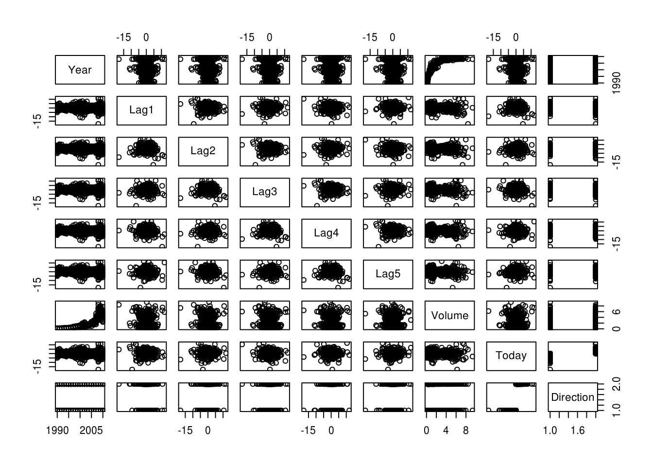
cor(subset(Weekly, select = -Direction)) Year Lag1 Lag2 Lag3 Lag4
Year 1.00000000 -0.032289274 -0.03339001 -0.03000649 -0.031127923
Lag1 -0.03228927 1.000000000 -0.07485305 0.05863568 -0.071273876
Lag2 -0.03339001 -0.074853051 1.00000000 -0.07572091 0.058381535
Lag3 -0.03000649 0.058635682 -0.07572091 1.00000000 -0.075395865
Lag4 -0.03112792 -0.071273876 0.05838153 -0.07539587 1.000000000
Lag5 -0.03051910 -0.008183096 -0.07249948 0.06065717 -0.075675027
Volume 0.84194162 -0.064951313 -0.08551314 -0.06928771 -0.061074617
Today -0.03245989 -0.075031842 0.05916672 -0.07124364 -0.007825873
Lag5 Volume Today
Year -0.030519101 0.84194162 -0.032459894
Lag1 -0.008183096 -0.06495131 -0.075031842
Lag2 -0.072499482 -0.08551314 0.059166717
Lag3 0.060657175 -0.06928771 -0.071243639
Lag4 -0.075675027 -0.06107462 -0.007825873
Lag5 1.000000000 -0.05851741 0.011012698
Volume -0.058517414 1.00000000 -0.033077783
Today 0.011012698 -0.03307778 1.000000000Year and Volume appear to have a relationship. No other patterns are discernible.
- Use the full data set to perform a logistic regression with
Directionas the response and the five lag variables plusVolumeas predictors. Use the summary function to print the results. Do any of the predictors appear to be statistically significant? If so, which ones?
logit_model <- glm(Direction ~ Lag1 + Lag2 + Lag3 + Lag4 + Lag5 + Volume,
                   data = Weekly,
                   family = binomial)
summary(logit_model)
Call:
glm(formula = Direction ~ Lag1 + Lag2 + Lag3 + Lag4 + Lag5 +
    Volume, family = binomial, data = Weekly)

Deviance Residuals:
    Min       1Q   Median       3Q      Max
-1.6949  -1.2565   0.9913   1.0849   1.4579

Coefficients:
            Estimate Std. Error z value Pr(>|z|)
(Intercept)  0.26686    0.08593   3.106   0.0019 **
Lag1        -0.04127    0.02641  -1.563   0.1181
Lag2         0.05844    0.02686   2.175   0.0296 *
Lag3        -0.01606    0.02666  -0.602   0.5469
Lag4        -0.02779    0.02646  -1.050   0.2937
Lag5        -0.01447    0.02638  -0.549   0.5833
Volume      -0.02274    0.03690  -0.616   0.5377
---
Signif. codes:  0 '***' 0.001 '**' 0.01 '*' 0.05 '.' 0.1 ' ' 1

(Dispersion parameter for binomial family taken to be 1)

    Null deviance: 1496.2  on 1088  degrees of freedom
Residual deviance: 1486.4  on 1082  degrees of freedom
AIC: 1500.4

Number of Fisher Scoring iterations: 4
Lag2 appears to have some statistical significance with a p-value of less than 0.05
- Compute the confusion matrix and overall fraction of correct predictions. Explain what the confusion matrix is telling you about the types of mistakes made by logistic regression.
We’ll write two functions so we don’t have to copy/paste code all over the place:
show_model_performance- Displays model performance.predict_glm_direction- Gets predictions as Up/Down class labels
# show confusion matrix from predicted class and observed class
show_model_performance <- function(predicted_status, observed_status) {
  confusion_matrix <- table(predicted_status,
                            observed_status,
                            dnn = c("Predicted Status", "Observed Status"))
  print(confusion_matrix)

  error_rate <- mean(predicted_status != observed_status)

  cat("\n") # \n means newline so it just prints a blank line
  cat("         Error Rate:", 100 * error_rate, "%\n")
  cat("Correctly Predicted:", 100 * (1-error_rate), "%\n")
  cat("False Positive Rate:", 100 * confusion_matrix[2,1] / sum(confusion_matrix[,1]), "%\n")
  cat("False Negative Rate:", 100 * confusion_matrix[1,2] / sum(confusion_matrix[,2]), "%\n")
}

# get prediction as Up/Down direction - only needed for GLM models
predict_glm_direction <- function(model, newdata = NULL) {
  predictions <- predict(model, newdata, type="response")
  return(as.factor(ifelse(predictions < 0.5, "Down", "Up")))
}
Now, all we need to do is call our functions to get the predictions and display model performance.
predicted_direction <- predict_glm_direction(logit_model)

show_model_performance(predicted_direction, Weekly$Direction)
Observed Status
Predicted Status Down Up
Down 54 48
Up 430 557
Error Rate: 43.89348 %
Correctly Predicted: 56.10652 %
False Positive Rate: 88.84298 %
False Negative Rate: 7.933884 %- Now fit the logistic regression model using a training data period from 1990 to 2008, with
Lag2as the only predictor. Compute the confusion matrix and the overall fraction of correct predictions for the held out data (that is, the data from 2009 and 2010).
train <- (Weekly$Year < 2009)
train_set <- Weekly[train, ]
test_set <- Weekly[!train, ]

logit_model <- glm(Direction ~ Lag2, data = Weekly, family = binomial, subset = train)

predicted_direction <- predict_glm_direction(logit_model, test_set)
show_model_performance(predicted_direction, test_set$Direction)
Observed Status
Predicted Status Down Up
Down 9 5
Up 34 56
Error Rate: 37.5 %
Correctly Predicted: 62.5 %
False Positive Rate: 79.06977 %
False Negative Rate: 8.196721 %- Repeat (d) using LDA.
library(MASS)

lda_model <- lda(Direction ~ Lag2, data = Weekly, subset = train)

predictions <- predict(lda_model, test_set, type="response")
show_model_performance(predictions$class, test_set$Direction)
Observed Status
Predicted Status Down Up
Down 9 5
Up 34 56
Error Rate: 37.5 %
Correctly Predicted: 62.5 %
False Positive Rate: 79.06977 %
False Negative Rate: 8.196721 %- Repeat (d) using QDA.
qda_model <- qda(Direction ~ Lag2, data = Weekly, subset = train)

predictions <- predict(qda_model, test_set, type="response")
show_model_performance(predictions$class, test_set$Direction)
Observed Status
Predicted Status Down Up
Down 0 0
Up 43 61
Error Rate: 41.34615 %
Correctly Predicted: 58.65385 %
False Positive Rate: 100 %
False Negative Rate: 0 %- Repeat (d) using KNN with K = 1.
library(class)

run_knn <- function(train, test, train_class, test_class, k) {
  set.seed(12345)
  predictions <- knn(train, test, train_class, k)

  cat("KNN: k =", k, "\n")
  show_model_performance(predictions, test_class)
}
train_matrix <- as.matrix(train_set$Lag2)
test_matrix <- as.matrix(test_set$Lag2)
run_knn(train_matrix, test_matrix, train_set$Direction, test_set$Direction, k = 1)KNN: k = 1
Observed Status
Predicted Status Down Up
Down 21 29
Up 22 32
Error Rate: 49.03846 %
Correctly Predicted: 50.96154 %
False Positive Rate: 51.16279 %
False Negative Rate: 47.54098 %- Which of these methods appears to provide the best results on this data?
Logistic regression and LDA methods provide similar test error rates.
- Experiment with different combinations of predictors, including possible transformations and interactions for each of the methods. Report the variables, method, and associated confusion matrix that appears to provide the best results on the held out data. Note that you should also experiment with values for K in the KNN classifier.
# Logistic regression with Lag1 * Lag2 interaction
logit_model <- glm(Direction ~ Lag1 * Lag2, data = Weekly, family = binomial, subset = train)

predicted_direction <- predict_glm_direction(logit_model, test_set)
show_model_performance(predicted_direction, test_set$Direction)
Observed Status
Predicted Status Down Up
Down 7 8
Up 36 53
Error Rate: 42.30769 %
Correctly Predicted: 57.69231 %
False Positive Rate: 83.72093 %
False Negative Rate: 13.11475 %# LDA with Lag1 * Lag2 interaction
lda_model <- lda(Direction ~ Lag1 * Lag2, data = Weekly, subset = train)
predictions <- predict(lda_model, test_set, type="response")
show_model_performance(predictions$class, test_set$Direction) Observed Status
Predicted Status Down Up
Down 7 8
Up 36 53
Error Rate: 42.30769 %
Correctly Predicted: 57.69231 %
False Positive Rate: 83.72093 %
False Negative Rate: 13.11475 %# QDA with sqrt(abs(Lag2))
qda_model <- qda(Direction ~ Lag2 + sqrt(abs(Lag2)), data = Weekly, subset = train)
predictions <- predict(qda_model, test_set, type="response")
show_model_performance(predictions$class, test_set$Direction) Observed Status
Predicted Status Down Up
Down 12 13
Up 31 48
Error Rate: 42.30769 %
Correctly Predicted: 57.69231 %
False Positive Rate: 72.09302 %
False Negative Rate: 21.31148 %# KNN k =10
run_knn(train_matrix, test_matrix, train_set$Direction, test_set$Direction, k = 10)KNN: k = 10
Observed Status
Predicted Status Down Up
Down 18 21
Up 25 40
Error Rate: 44.23077 %
Correctly Predicted: 55.76923 %
False Positive Rate: 58.13953 %
False Negative Rate: 34.42623 %# KNN k = 100
run_knn(train_matrix, test_matrix, train_set$Direction, test_set$Direction, k = 100)KNN: k = 100
Observed Status
Predicted Status Down Up
Down 10 13
Up 33 48
Error Rate: 44.23077 %
Correctly Predicted: 55.76923 %
False Positive Rate: 76.74419 %
False Negative Rate: 21.31148 %Out of these permutations, the original LDA and logistic regression have better performance in terms of test error rate.
3.2.2 Exercise
In this problem, you will develop a model to predict whether a given car gets high or low gas mileage based on the Auto dataset from the ISLR package.
- Create a binary variable,
mpg01, that contains a 1 ifmpgcontains a value above its median, and a 0 ifmpgcontains a value below its median. You can compute the median using themedian()function. Note you may find it helpful to use thedata.frame()function to create a single data set containing bothmpg01and the otherAutovariables.
We can use ifelse() to create a variable with values of 0 or 1, or we could just use the logical TRUE/FALSE which is even easier to create.
Auto$mpg01 <- Auto$mpg > median(Auto$mpg)Now let’s see what mpg01 looks like:
head(Auto$mpg01, n = 20) [1] FALSE FALSE FALSE FALSE FALSE FALSE FALSE FALSE FALSE FALSE FALSE
[12] FALSE FALSE FALSE TRUE FALSE FALSE FALSE TRUE TRUE- Explore the data graphically in order to investigate the association between
mpg01and the other features. Which of the other features seem most likely to be useful in predictingmpg01? Scatterplots and boxplots may be useful tools to answer this question. Describe your findings.
cor(subset(Auto, select = -name)) mpg cylinders displacement horsepower weight
mpg 1.0000000 -0.7776175 -0.8051269 -0.7784268 -0.8322442
cylinders -0.7776175 1.0000000 0.9508233 0.8429834 0.8975273
displacement -0.8051269 0.9508233 1.0000000 0.8972570 0.9329944
horsepower -0.7784268 0.8429834 0.8972570 1.0000000 0.8645377
weight -0.8322442 0.8975273 0.9329944 0.8645377 1.0000000
acceleration 0.4233285 -0.5046834 -0.5438005 -0.6891955 -0.4168392
year 0.5805410 -0.3456474 -0.3698552 -0.4163615 -0.3091199
origin 0.5652088 -0.5689316 -0.6145351 -0.4551715 -0.5850054
mpg01 0.8369392 -0.7591939 -0.7534766 -0.6670526 -0.7577566
acceleration year origin mpg01
mpg 0.4233285 0.5805410 0.5652088 0.8369392
cylinders -0.5046834 -0.3456474 -0.5689316 -0.7591939
displacement -0.5438005 -0.3698552 -0.6145351 -0.7534766
horsepower -0.6891955 -0.4163615 -0.4551715 -0.6670526
weight -0.4168392 -0.3091199 -0.5850054 -0.7577566
acceleration 1.0000000 0.2903161 0.2127458 0.3468215
year 0.2903161 1.0000000 0.1815277 0.4299042
origin 0.2127458 0.1815277 1.0000000 0.5136984
mpg01 0.3468215 0.4299042 0.5136984 1.0000000pairs(Auto) # not very useful since mpg01 is binary but let's see what we get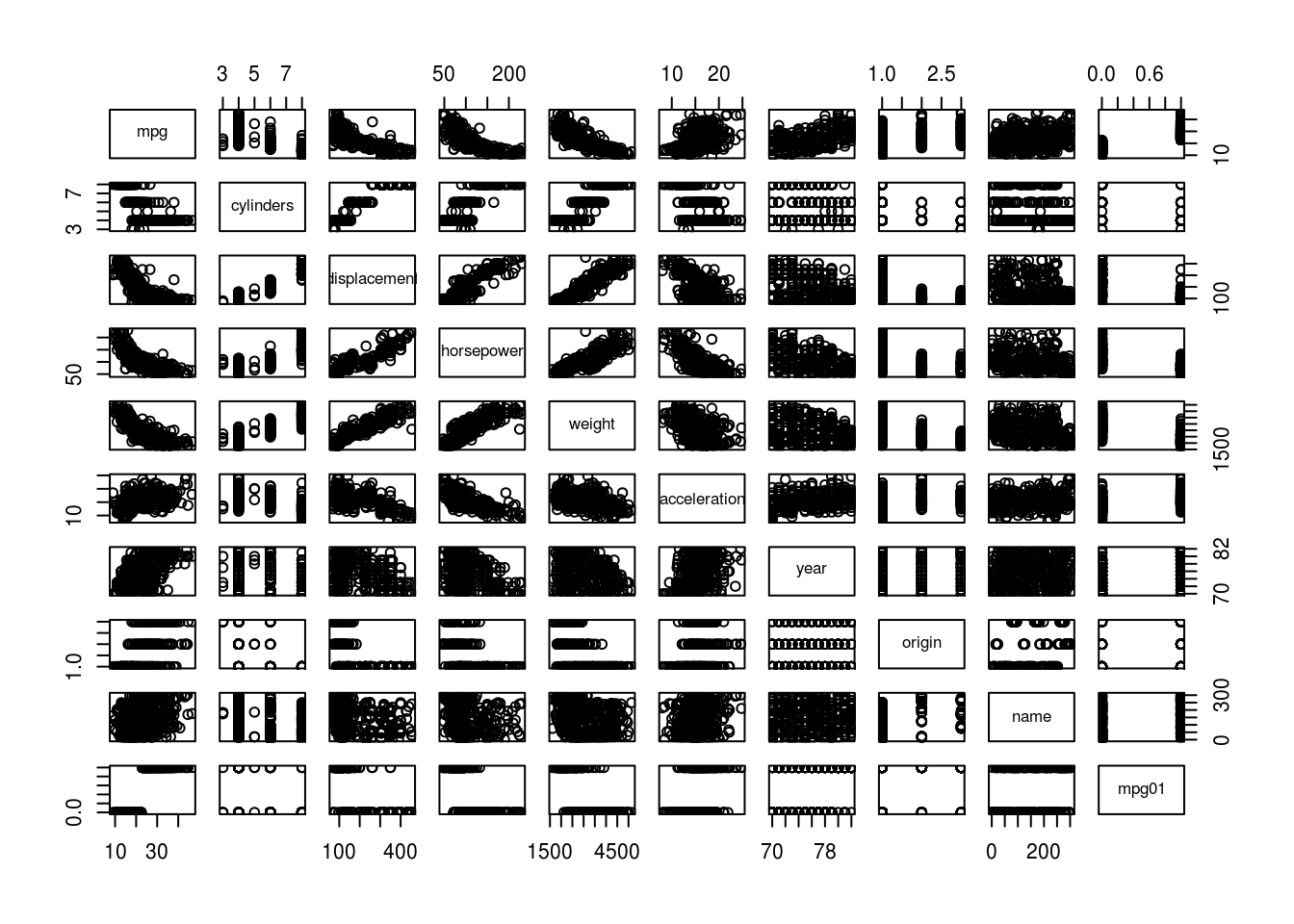
cylinders, weight, displacement, horsepower (and mpg itself) seem most likely to be useful in predicting mpg01
- Split the data into a training set and a test set.
train <- sample(nrow(Auto) * 0.7)
train_set <- Auto[train, ]
test_set <- Auto[-train, ]- Perform LDA on the training data in order to predict
mpg01using the variables that seemed most associated withmpg01in (b). What is the test error of the model obtained?
lda_model <- lda(mpg01 ~ cylinders + weight + displacement + horsepower,
                 data = Auto,
                 subset = train)

predictions <- predict(lda_model, test_set)
show_model_performance(predictions$class, test_set$mpg01)
Observed Status
Predicted Status FALSE TRUE
FALSE 18 16
TRUE 2 82
Error Rate: 15.25424 %
Correctly Predicted: 84.74576 %
False Positive Rate: 10 %
False Negative Rate: 16.32653 %- Perform QDA on the training data in order to predict
mpg01using the variables that seemed most associated withmpg01in (b). What is the test error of the model obtained?
qda_model <- qda(mpg01 ~ cylinders + weight + displacement + horsepower,
                 data = Auto,
                 subset = train)

predictions <- predict(qda_model, test_set)
show_model_performance(predictions$class, test_set$mpg01)
Observed Status
Predicted Status FALSE TRUE
FALSE 18 19
TRUE 2 79
Error Rate: 17.79661 %
Correctly Predicted: 82.20339 %
False Positive Rate: 10 %
False Negative Rate: 19.38776 %- Perform logistic regression on the training data in order to predict
mpg01using the variables that seemed most associated withmpg01in (b). What is the test error of the model obtained?
logit_model <- glm(mpg01 ~ cylinders + weight + displacement + horsepower,
                   data = Auto,
                   family = binomial,
                   subset = train)

predictions <- predict(logit_model, test_set, type = "response")
show_model_performance(predictions > 0.5, test_set$mpg01)
Observed Status
Predicted Status FALSE TRUE
FALSE 20 21
TRUE 0 77
Error Rate: 17.79661 %
Correctly Predicted: 82.20339 %
False Positive Rate: 0 %
False Negative Rate: 21.42857 %- Perform KNN on the training data, with several values of K, in order to predict
mpg01. Use only the variables that seemed most associated withmpg01in (b). What test errors do you obtain? Which value of K seems to perform the best on this data set?
vars <- c("cylinders", "weight", "displacement", "horsepower")
train_matrix <- as.matrix(train_set[, vars])
test_matrix <- as.matrix(test_set[, vars])

predictions <- knn(train_matrix, test_matrix, train_set$mpg01, 1)

run_knn(train_matrix, test_matrix, train_set$mpg01, test_set$mpg01, k = 1)
KNN: k = 1
Observed Status
Predicted Status FALSE TRUE
FALSE 18 24
TRUE 2 74
Error Rate: 22.0339 %
Correctly Predicted: 77.9661 %
False Positive Rate: 10 %
False Negative Rate: 24.4898 %run_knn(train_matrix, test_matrix, train_set$mpg01, test_set$mpg01, k = 10)KNN: k = 10
Observed Status
Predicted Status FALSE TRUE
FALSE 20 22
TRUE 0 76
Error Rate: 18.64407 %
Correctly Predicted: 81.35593 %
False Positive Rate: 0 %
False Negative Rate: 22.44898 %run_knn(train_matrix, test_matrix, train_set$mpg01, test_set$mpg01, k = 100)KNN: k = 100
Observed Status
Predicted Status FALSE TRUE
FALSE 20 25
TRUE 0 73
Error Rate: 21.18644 %
Correctly Predicted: 78.81356 %
False Positive Rate: 0 %
False Negative Rate: 25.5102 %3.2.3 Exercise
This problem involves writing functions.
Write a function
calc_square(), that returns the result of raising a number to the 2nd power. For example, callingcalc_square(5)should return the result of \(5^2\) or 25.Hint: Recall that
x^araisesxto the powera. Use theprint()function to output the result.
calc_square <- function(x) {
  return(x^2)
}
We can test our function like this:
calc_square(3)[1] 9calc_square(5)[1] 25- Write a new function
calc_power(), that allows you to pass any two numbers,xanda, and prints out the value ofx^a. For example, you should be able to callcalc_power(3,8)and your function should return \(3^8\) or 6561.
calc_power <- function(x,a) {
  return(x^a)
}- Using the
calc_power()function that you just wrote, compute \(10^3\), \(8^{17}\), and \(131^3\).
calc_power(10, 3)[1] 1000calc_power(8, 17)[1] 2.2518e+15calc_power(131, 3)[1] 2248091- Now using the
calc_power()function, create a plot of \(f(x) = x^2\). The \(x\)-axis should display a range of integers from 1 to 10, and the \(y\)-axis should display \(x^2\). Label the axes appropriately, and use an appropriate title for the figure. Consider displaying either the \(x\)-axis, the \(y\)-axis, or both on the log-scale. You can do this by usinglog="x",log="y", orlog="xy"as arguments to theplot()function.
x <- 1:10
plot(x, calc_power(x, 2),
     log="xy", ylab="Log of y = x^2", xlab="Log of x",
     main="Log of x^2 versus Log of x")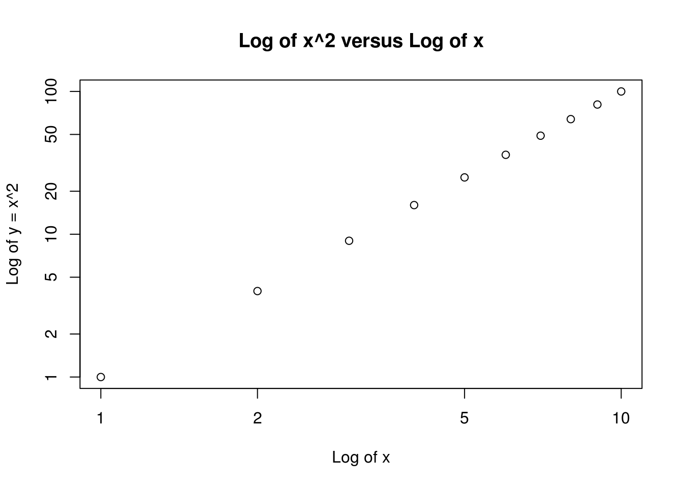
- Write a function
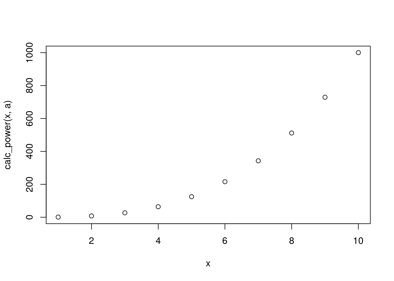
plot_power(), that allows you to create a plot ofxagainstx^afor a fixedaand for a range of values ofx. For instance:
plot_power <- function(x, a) {
  plot(x, calc_power(x, a))
}
The result should be a plot with an \(x\)-axis taking on values \(1,2,\dots ,10\), and a \(y\)-axis taking on values \(1^3,2^3,\dots ,10^3\).
plot_power(1:10, 3)