Advanced Quantitative Methods

6.2 Solutions

library(ISLR)
library(e1071)

6.2.1 Exercise

This problem involves the OJ data set which is part of the ISLR package.

Create a training set containing a random sample of 800 observations, and a test set containing the remaining observations.

set.seed(112233)

train <- sample(nrow(OJ), 800)
OJ_train <- OJ[train, ]
OJ_test <- OJ[-train, ]

Fit a support vector classifier to the training data using cost=0.01, with Purchase as the response and the other variables as predictors. Use the summary() function to produce summary statistics, and describe the results obtained.

svm_linear <- svm(Purchase ~ . , kernel = "linear", data = OJ_train, cost = 0.01)
summary(svm_linear)


Call:
svm(formula = Purchase ~ ., data = OJ_train, kernel = "linear", 
    cost = 0.01)


Parameters:
   SVM-Type:  C-classification 
 SVM-Kernel:  linear 
       cost:  0.01 
      gamma:  0.05555556 

Number of Support Vectors:  432

 ( 217 215 )


Number of Classes:  2 

Levels: 
 CH MM

Support vector classifier creates 432 support vectors out of 800 training points. Out of these, 217 belong to level CH and remaining 215 belong to level MM.

What are the training and test error rates?

# calculate error rate
calc_error_rate <- function(svm_model, dataset, true_classes) {
  confusion_matrix <- table(predict(svm_model, dataset), true_classes)
  return(1 - sum(diag(confusion_matrix)) / sum(confusion_matrix))
}

cat("Training Error Rate:", 100 * calc_error_rate(svm_linear, OJ_train, OJ_train$Purchase), "%\n")

Training Error Rate: 16 %

cat("Test Error Rate:", 100 * calc_error_rate(svm_linear, OJ_test, OJ_test$Purchase), "%\n")

Test Error Rate: 18.88889 %

Use the tune() function to select an optimal cost. Consider values in the range 0.01 to 10.

set.seed(112233)

svm_tune <- tune(svm, Purchase ~ . , data = OJ, kernel = "linear", 
                  ranges = list(cost = seq(0.01, 10, length = 100)))
summary(svm_tune)


Parameter tuning of 'svm':

- sampling method: 10-fold cross validation 

- best parameters:
     cost
 3.743636

- best performance: 0.1616822 

- Detailed performance results:
          cost     error dispersion
1    0.0100000 0.1663551 0.03463412
2    0.1109091 0.1672897 0.02767155
3    0.2118182 0.1663551 0.03013928
4    0.3127273 0.1672897 0.03280656
5    0.4136364 0.1672897 0.03280656
6    0.5145455 0.1672897 0.03280656
7    0.6154545 0.1672897 0.03280656
8    0.7163636 0.1682243 0.03355243
9    0.8172727 0.1682243 0.03355243
10   0.9181818 0.1682243 0.03355243
11   1.0190909 0.1672897 0.03509343
12   1.1200000 0.1672897 0.03509343
13   1.2209091 0.1682243 0.03579167
14   1.3218182 0.1663551 0.03463412
15   1.4227273 0.1644860 0.03691293
16   1.5236364 0.1635514 0.03692607
17   1.6245455 0.1635514 0.03692607
18   1.7254545 0.1635514 0.03692607
19   1.8263636 0.1635514 0.03692607
20   1.9272727 0.1635514 0.03692607
21   2.0281818 0.1644860 0.03664907
22   2.1290909 0.1644860 0.03664907
23   2.2300000 0.1644860 0.03664907
24   2.3309091 0.1644860 0.03502422
25   2.4318182 0.1635514 0.03531397
26   2.5327273 0.1635514 0.03531397
27   2.6336364 0.1635514 0.03531397
28   2.7345455 0.1644860 0.03502422
29   2.8354545 0.1644860 0.03502422
30   2.9363636 0.1644860 0.03502422
31   3.0372727 0.1644860 0.03502422
32   3.1381818 0.1644860 0.03502422
33   3.2390909 0.1635514 0.03531397
34   3.3400000 0.1644860 0.03502422
35   3.4409091 0.1626168 0.03389775
36   3.5418182 0.1635514 0.03419704
37   3.6427273 0.1626168 0.03389775
38   3.7436364 0.1616822 0.03580522
39   3.8445455 0.1644860 0.03611558
40   3.9454545 0.1644860 0.03611558
41   4.0463636 0.1635514 0.03796280
42   4.1472727 0.1635514 0.03796280
43   4.2481818 0.1635514 0.03796280
44   4.3490909 0.1654206 0.03687347
45   4.4500000 0.1644860 0.03870959
46   4.5509091 0.1654206 0.03687347
47   4.6518182 0.1635514 0.03770629
48   4.7527273 0.1635514 0.03770629
49   4.8536364 0.1635514 0.03770629
50   4.9545455 0.1644860 0.03795001
51   5.0554545 0.1654206 0.03765478
52   5.1563636 0.1654206 0.03765478
53   5.2572727 0.1654206 0.03765478
54   5.3581818 0.1654206 0.03892211
55   5.4590909 0.1663551 0.04008899
56   5.5600000 0.1663551 0.04008899
57   5.6609091 0.1654206 0.04063003
58   5.7618182 0.1654206 0.04063003
59   5.8627273 0.1663551 0.03885973
60   5.9636364 0.1663551 0.04151609
61   6.0645455 0.1663551 0.04151609
62   6.1654545 0.1663551 0.04151609
63   6.2663636 0.1663551 0.04151609
64   6.3672727 0.1654206 0.04039046
65   6.4681818 0.1663551 0.04151609
66   6.5690909 0.1663551 0.03860918
67   6.6700000 0.1663551 0.04151609
68   6.7709091 0.1663551 0.04151609
69   6.8718182 0.1663551 0.04151609
70   6.9727273 0.1672897 0.03976084
71   7.0736364 0.1672897 0.03976084
72   7.1745455 0.1672897 0.03976084
73   7.2754545 0.1672897 0.03976084
74   7.3763636 0.1672897 0.03976084
75   7.4772727 0.1663551 0.03860918
76   7.5781818 0.1672897 0.03976084
77   7.6790909 0.1672897 0.03976084
78   7.7800000 0.1672897 0.03976084
79   7.8809091 0.1672897 0.03976084
80   7.9818182 0.1672897 0.03976084
81   8.0827273 0.1672897 0.03976084
82   8.1836364 0.1672897 0.03976084
83   8.2845455 0.1672897 0.03976084
84   8.3854545 0.1672897 0.03976084
85   8.4863636 0.1672897 0.03976084
86   8.5872727 0.1672897 0.03976084
87   8.6881818 0.1672897 0.03976084
88   8.7890909 0.1672897 0.03976084
89   8.8900000 0.1672897 0.03976084
90   8.9909091 0.1672897 0.03976084
91   9.0918182 0.1672897 0.03976084
92   9.1927273 0.1672897 0.03976084
93   9.2936364 0.1672897 0.03976084
94   9.3945455 0.1672897 0.03976084
95   9.4954545 0.1672897 0.03976084
96   9.5963636 0.1672897 0.03976084
97   9.6972727 0.1672897 0.03976084
98   9.7981818 0.1672897 0.03976084
99   9.8990909 0.1672897 0.03976084
100 10.0000000 0.1672897 0.03976084

Tuning shows that optimal cost is 3.7436364.

Compute the training and test error rates using this new value for cost.

svm_linear <- svm(Purchase ~ . , kernel = "linear", 
                  data = OJ_train, cost = svm_tune$best.parameters$cost)

cat("Training Error Rate:", 100 * calc_error_rate(svm_linear, OJ_train, OJ_train$Purchase), "%\n")

Training Error Rate: 15.875 %

cat("Test Error Rate:", 100 * calc_error_rate(svm_linear, OJ_test, OJ_test$Purchase), "%\n")

Test Error Rate: 19.25926 %

Repeat parts (b) through (e) using a support vector machine with a radial kernel. Use the default value for gamma.

set.seed(112233)

svm_radial <- svm(Purchase ~ . , data = OJ_train, kernel = "radial")
summary(svm_radial)


Call:
svm(formula = Purchase ~ ., data = OJ_train, kernel = "radial")


Parameters:
   SVM-Type:  C-classification 
 SVM-Kernel:  radial 
       cost:  1 
      gamma:  0.05555556 

Number of Support Vectors:  364

 ( 183 181 )


Number of Classes:  2 

Levels: 
 CH MM

cat("Training Error Rate:", 100 * calc_error_rate(svm_radial, OJ_train, OJ_train$Purchase), "%\n")

Training Error Rate: 14 %

cat("Test Error Rate:", 100 * calc_error_rate(svm_radial, OJ_test, OJ_test$Purchase), "%\n")

Test Error Rate: 21.85185 %

The radial basis kernel with default gamma creates 364 support vectors, out of which, 183 belong to level CH and remaining 183 belong to level MM.

set.seed(112233)

svm_tune <- tune(svm, Purchase ~ . , data = OJ_train, kernel = "radial",
                  ranges = list(cost = seq(0.01, 10, length = 100)))
summary(svm_tune)


Parameter tuning of 'svm':

- sampling method: 10-fold cross validation 

- best parameters:
      cost
 0.4136364

- best performance: 0.1575 

- Detailed performance results:
          cost   error dispersion
1    0.0100000 0.39750 0.04816061
2    0.1109091 0.17375 0.04803428
3    0.2118182 0.17000 0.04721405
4    0.3127273 0.16250 0.04208127
5    0.4136364 0.15750 0.03872983
6    0.5145455 0.16625 0.03866254
7    0.6154545 0.17000 0.03917553
8    0.7163636 0.16750 0.03641962
9    0.8172727 0.16375 0.03408018
10   0.9181818 0.16375 0.03557562
11   1.0190909 0.16500 0.03525699
12   1.1200000 0.16375 0.03251602
13   1.2209091 0.16250 0.03535534
14   1.3218182 0.16500 0.03622844
15   1.4227273 0.16625 0.03488573
16   1.5236364 0.17125 0.03775377
17   1.6245455 0.17250 0.03899786
18   1.7254545 0.17000 0.04216370
19   1.8263636 0.16875 0.04259385
20   1.9272727 0.16750 0.04216370
21   2.0281818 0.16875 0.04007372
22   2.1290909 0.17000 0.04133199
23   2.2300000 0.17125 0.04084609
24   2.3309091 0.17125 0.04084609
25   2.4318182 0.17125 0.04084609
26   2.5327273 0.17125 0.04084609
27   2.6336364 0.17250 0.03899786
28   2.7345455 0.17250 0.03899786
29   2.8354545 0.17125 0.03955042
30   2.9363636 0.16875 0.04050463
31   3.0372727 0.16875 0.04050463
32   3.1381818 0.16875 0.04050463
33   3.2390909 0.16750 0.04005205
34   3.3400000 0.16750 0.04005205
35   3.4409091 0.16750 0.04005205
36   3.5418182 0.16750 0.04005205
37   3.6427273 0.16875 0.04177070
38   3.7436364 0.16875 0.04177070
39   3.8445455 0.16875 0.04177070
40   3.9454545 0.17000 0.04174992
41   4.0463636 0.17000 0.04174992
42   4.1472727 0.17000 0.04174992
43   4.2481818 0.17000 0.04174992
44   4.3490909 0.17250 0.04281744
45   4.4500000 0.17250 0.04281744
46   4.5509091 0.17125 0.04291869
47   4.6518182 0.17250 0.04594683
48   4.7527273 0.17375 0.04543387
49   4.8536364 0.17375 0.04543387
50   4.9545455 0.17375 0.04543387
51   5.0554545 0.17375 0.04543387
52   5.1563636 0.17375 0.04543387
53   5.2572727 0.17375 0.04543387
54   5.3581818 0.17375 0.04543387
55   5.4590909 0.17250 0.04706674
56   5.5600000 0.17250 0.04706674
57   5.6609091 0.17250 0.04706674
58   5.7618182 0.17250 0.04706674
59   5.8627273 0.17250 0.04706674
60   5.9636364 0.17250 0.04706674
61   6.0645455 0.17250 0.04706674
62   6.1654545 0.17250 0.04706674
63   6.2663636 0.17250 0.04706674
64   6.3672727 0.17250 0.04706674
65   6.4681818 0.17250 0.04706674
66   6.5690909 0.17250 0.04706674
67   6.6700000 0.17250 0.04706674
68   6.7709091 0.17250 0.04706674
69   6.8718182 0.17250 0.04706674
70   6.9727273 0.17250 0.04706674
71   7.0736364 0.17375 0.04543387
72   7.1745455 0.17375 0.04543387
73   7.2754545 0.17375 0.04543387
74   7.3763636 0.17375 0.04543387
75   7.4772727 0.17375 0.04543387
76   7.5781818 0.17375 0.04543387
77   7.6790909 0.17375 0.04543387
78   7.7800000 0.17375 0.04543387
79   7.8809091 0.17375 0.04543387
80   7.9818182 0.17375 0.04543387
81   8.0827273 0.17375 0.04543387
82   8.1836364 0.17375 0.04543387
83   8.2845455 0.17375 0.04543387
84   8.3854545 0.17250 0.04440971
85   8.4863636 0.17250 0.04440971
86   8.5872727 0.17250 0.04440971
87   8.6881818 0.17250 0.04440971
88   8.7890909 0.17250 0.04440971
89   8.8900000 0.17250 0.04440971
90   8.9909091 0.17250 0.04440971
91   9.0918182 0.17250 0.04440971
92   9.1927273 0.17250 0.04440971
93   9.2936364 0.17250 0.04440971
94   9.3945455 0.17250 0.04440971
95   9.4954545 0.17125 0.04489571
96   9.5963636 0.17125 0.04489571
97   9.6972727 0.17250 0.04479893
98   9.7981818 0.17250 0.04479893
99   9.8990909 0.17375 0.04427267
100 10.0000000 0.17375 0.04427267

svm_radial <- svm(Purchase ~ . , data = OJ_train, kernel = "radial",
                   cost = svm_tune$best.parameters$cost)

cat("Training Error Rate:", 100 * calc_error_rate(svm_radial, OJ_train, OJ_train$Purchase), "%\n")

Training Error Rate: 14 %

cat("Test Error Rate:", 100 * calc_error_rate(svm_radial, OJ_test, OJ_test$Purchase), "%\n")

Test Error Rate: 21.11111 %

Repeat parts (b) through (e) using a support vector machine with a polynomial kernel. Set degree=2.

set.seed(112233)

svm_poly <- svm(Purchase ~ . , data = OJ_train, kernel = "poly", degree = 2)
summary(svm_poly)


Call:
svm(formula = Purchase ~ ., data = OJ_train, kernel = "poly", 
    degree = 2)


Parameters:
   SVM-Type:  C-classification 
 SVM-Kernel:  polynomial 
       cost:  1 
     degree:  2 
      gamma:  0.05555556 
     coef.0:  0 

Number of Support Vectors:  442

 ( 225 217 )


Number of Classes:  2 

Levels: 
 CH MM

cat("Training Error Rate:", 100 * calc_error_rate(svm_poly, OJ_train, OJ_train$Purchase), "%\n")

Training Error Rate: 16.75 %

cat("Test Error Rate:", 100 * calc_error_rate(svm_poly, OJ_test, OJ_test$Purchase), "%\n")

Test Error Rate: 22.96296 %

set.seed(112233)

svm_tune <- tune(svm, Purchase ~ . , data = OJ_train, kernel = "poly", 
                  degree = 2, ranges = list(cost = seq(0.01, 10, length = 100)))
summary(svm_tune)


Parameter tuning of 'svm':

- sampling method: 10-fold cross validation 

- best parameters:
     cost
 8.486364

- best performance: 0.1675 

- Detailed performance results:
          cost   error dispersion
1    0.0100000 0.38500 0.05394184
2    0.1109091 0.30000 0.05559027
3    0.2118182 0.22625 0.04839436
4    0.3127273 0.20125 0.04016027
5    0.4136364 0.20125 0.04143687
6    0.5145455 0.19500 0.03827895
7    0.6154545 0.19000 0.03717451
8    0.7163636 0.19250 0.04133199
9    0.8172727 0.18875 0.04101575
10   0.9181818 0.19000 0.04116363
11   1.0190909 0.18500 0.04031129
12   1.1200000 0.18375 0.03682259
13   1.2209091 0.18500 0.03899786
14   1.3218182 0.18375 0.04084609
15   1.4227273 0.18250 0.04297932
16   1.5236364 0.18250 0.04571956
17   1.6245455 0.18125 0.04340139
18   1.7254545 0.18000 0.04297932
19   1.8263636 0.17750 0.04322101
20   1.9272727 0.17500 0.04082483
21   2.0281818 0.17375 0.04101575
22   2.1290909 0.17375 0.04101575
23   2.2300000 0.17250 0.03944053
24   2.3309091 0.17125 0.04210189
25   2.4318182 0.17000 0.03917553
26   2.5327273 0.17000 0.03736085
27   2.6336364 0.17000 0.03736085
28   2.7345455 0.17000 0.03736085
29   2.8354545 0.16875 0.04007372
30   2.9363636 0.16875 0.03963812
31   3.0372727 0.16875 0.04218428
32   3.1381818 0.17000 0.04456581
33   3.2390909 0.17125 0.04528076
34   3.3400000 0.17000 0.04417453
35   3.4409091 0.17000 0.04417453
36   3.5418182 0.16875 0.04497299
37   3.6427273 0.17000 0.04609772
38   3.7436364 0.17000 0.04609772
39   3.8445455 0.17000 0.04609772
40   3.9454545 0.17000 0.04609772
41   4.0463636 0.16875 0.04686342
42   4.1472727 0.16875 0.04686342
43   4.2481818 0.16875 0.04686342
44   4.3490909 0.17000 0.04609772
45   4.4500000 0.17000 0.04609772
46   4.5509091 0.17000 0.04609772
47   4.6518182 0.17000 0.04609772
48   4.7527273 0.16875 0.04686342
49   4.8536364 0.16875 0.04686342
50   4.9545455 0.16875 0.04686342
51   5.0554545 0.16875 0.04686342
52   5.1563636 0.17000 0.04721405
53   5.2572727 0.17000 0.04721405
54   5.3581818 0.17250 0.04556741
55   5.4590909 0.17125 0.04678927
56   5.5600000 0.16875 0.04723243
57   5.6609091 0.17000 0.04972145
58   5.7618182 0.17125 0.05138701
59   5.8627273 0.17125 0.05138701
60   5.9636364 0.17125 0.05138701
61   6.0645455 0.17125 0.05138701
62   6.1654545 0.17250 0.05163978
63   6.2663636 0.17250 0.05163978
64   6.3672727 0.17375 0.05084358
65   6.4681818 0.17375 0.05084358
66   6.5690909 0.17375 0.05084358
67   6.6700000 0.17375 0.05084358
68   6.7709091 0.17375 0.05084358
69   6.8718182 0.17250 0.05296750
70   6.9727273 0.17000 0.05277047
71   7.0736364 0.17125 0.05369991
72   7.1745455 0.17000 0.05210833
73   7.2754545 0.17000 0.05210833
74   7.3763636 0.16875 0.05344065
75   7.4772727 0.17000 0.05277047
76   7.5781818 0.17000 0.05277047
77   7.6790909 0.16875 0.05344065
78   7.7800000 0.16875 0.05344065
79   7.8809091 0.16875 0.05344065
80   7.9818182 0.16875 0.05344065
81   8.0827273 0.16875 0.05344065
82   8.1836364 0.16875 0.05344065
83   8.2845455 0.16875 0.05344065
84   8.3854545 0.16875 0.05344065
85   8.4863636 0.16750 0.05244044
86   8.5872727 0.16750 0.05244044
87   8.6881818 0.16875 0.05408648
88   8.7890909 0.16875 0.05408648
89   8.8900000 0.16875 0.05408648
90   8.9909091 0.17000 0.05502525
91   9.0918182 0.17125 0.05744865
92   9.1927273 0.17125 0.05744865
93   9.2936364 0.17125 0.05744865
94   9.3945455 0.17125 0.05744865
95   9.4954545 0.17125 0.05744865
96   9.5963636 0.17000 0.05809475
97   9.6972727 0.17000 0.05809475
98   9.7981818 0.17000 0.05809475
99   9.8990909 0.16875 0.05899918
100 10.0000000 0.16875 0.05899918

svm_poly <- svm(Purchase ~ . , data = OJ_train, kernel = "poly", 
                 degree = 2, cost = svm_tune$best.parameters$cost)

cat("Training Error Rate:", 100 * calc_error_rate(svm_poly, OJ_train, OJ_train$Purchase), "%\n")

Training Error Rate: 14.125 %

cat("Test Error Rate:", 100 * calc_error_rate(svm_poly, OJ_test, OJ_test$Purchase), "%\n")

Test Error Rate: 21.48148 %

Overall, which approach seems to give the best results on this data?

Overall, radial basis kernel seems to be producing minimum misclassification error on training set but the linear kernel performs better on test data.

6.2.2 Exercise

In this problem, you will generate simulated data, and then perform PCA and K-means clustering on the data.

Generate a simulated data set with 20 observations in each of three classes (i.e. 60 observations total), and 50 variables. Hint: There are a number of functions in R that you can use to generate data. One example is the rnorm() function; runif() is another option. Be sure to add a mean shift to the observations in each class so that there are three distinct classes.

set.seed(11111)

x <- matrix(rnorm(20*3*50, mean=c(-4, 0, 4), sd=1), ncol=50)

The concept here is to separate the three classes amongst two dimensions.

Perform PCA on the 60 observations and plot the first two principal component score vectors. Use a different color to indicate the observations in each of the three classes. If the three classes appear separated in this plot, then continue on to part (c). If not, then return to part (a) and modify the simulation so that there is greater separation between the three classes. Do not continue to part (c) until the three classes show at least some separation in the first two principal component score vectors.

pca_model <- prcomp(x)
summary(pca_model)

Importance of components:
                           PC1     PC2     PC3     PC4    PC5     PC6
Standard deviation     23.3848 1.89806 1.77504 1.70329 1.6367 1.60229
Proportion of Variance  0.9185 0.00605 0.00529 0.00487 0.0045 0.00431
Cumulative Proportion   0.9185 0.92458 0.92987 0.93474 0.9392 0.94356
                          PC7     PC8     PC9    PC10    PC11    PC12
Standard deviation     1.5426 1.52814 1.45164 1.43140 1.40337 1.29265
Proportion of Variance 0.0040 0.00392 0.00354 0.00344 0.00331 0.00281
Cumulative Proportion  0.9476 0.95147 0.95501 0.95846 0.96176 0.96457
                          PC13    PC14    PC15    PC16    PC17    PC18
Standard deviation     1.26190 1.23964 1.17206 1.14254 1.10980 1.07022
Proportion of Variance 0.00267 0.00258 0.00231 0.00219 0.00207 0.00192
Cumulative Proportion  0.96725 0.96983 0.97213 0.97433 0.97640 0.97832
                         PC19    PC20    PC21    PC22    PC23    PC24
Standard deviation     1.0646 1.00376 0.95937 0.88838 0.88768 0.87603
Proportion of Variance 0.0019 0.00169 0.00155 0.00133 0.00132 0.00129
Cumulative Proportion  0.9802 0.98192 0.98346 0.98479 0.98611 0.98740
                          PC25    PC26   PC27    PC28    PC29    PC30
Standard deviation     0.83881 0.82276 0.8105 0.79896 0.73975 0.72993
Proportion of Variance 0.00118 0.00114 0.0011 0.00107 0.00092 0.00089
Cumulative Proportion  0.98858 0.98972 0.9908 0.99189 0.99281 0.99371
                         PC31    PC32    PC33    PC34    PC35   PC36
Standard deviation     0.6919 0.64788 0.61886 0.58353 0.56437 0.5483
Proportion of Variance 0.0008 0.00071 0.00064 0.00057 0.00053 0.0005
Cumulative Proportion  0.9945 0.99522 0.99586 0.99643 0.99697 0.9975
                          PC37    PC38    PC39   PC40    PC41   PC42
Standard deviation     0.51403 0.46435 0.43044 0.4256 0.40557 0.3419
Proportion of Variance 0.00044 0.00036 0.00031 0.0003 0.00028 0.0002
Cumulative Proportion  0.99792 0.99828 0.99859 0.9989 0.99917 0.9994
                          PC43    PC44    PC45    PC46    PC47    PC48
Standard deviation     0.33042 0.26632 0.25911 0.23286 0.17740 0.14808
Proportion of Variance 0.00018 0.00012 0.00011 0.00009 0.00005 0.00004
Cumulative Proportion  0.99955 0.99967 0.99978 0.99987 0.99993 0.99996
                          PC49    PC50
Standard deviation     0.12686 0.07922
Proportion of Variance 0.00003 0.00001
Cumulative Proportion  0.99999 1.00000

plot(pca_model$x[,1:2], col=2:4, xlab="Z1", ylab="Z2", pch=19)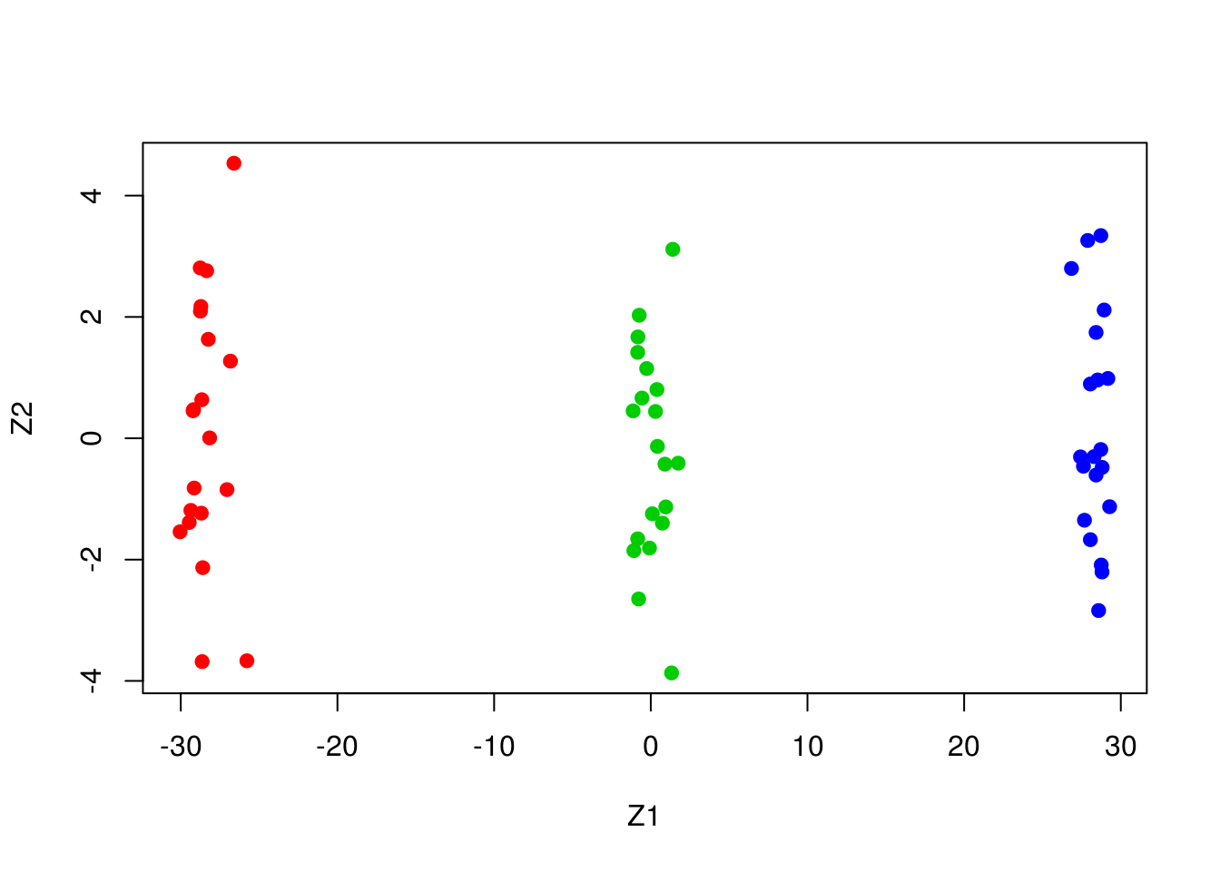

Perform \(K\)-means clustering of the observations with \(K = 3\). How well do the clusters that you obtained in \(K\)-means clustering compare to the true class labels?

Hint: You can use the table() function in R to compare the true class labels to the class labels obtained by clustering. Be careful how you interpret the results: \(K\)-means clustering will arbitrarily number the clusters, so you cannot simply check whether the true class labels and clustering labels are the same.

kmean_model <- kmeans(x, 3, nstart=20)
table(kmean_model$cluster, rep(1:3, 20))

Perfect match.

Perform \(K\)-means clustering with \(K = 2\). Describe your results.

kmean_model <- kmeans(x, 2, nstart=20)
kmean_model$cluster

 [1] 2 1 1 2 1 1 2 1 1 2 1 1 2 1 1 2 1 1 2 1 1 2 1 1 2 1 1 2 1 1 2 1 1 2 1
[36] 1 2 1 1 2 1 1 2 1 1 2 1 1 2 1 1 2 1 1 2 1 1 2 1 1

All of one previous class absorbed into a single class.

Now perform \(K\)-means clustering with \(K = 4\), and describe your results.

kmean_model <- kmeans(x, 4, nstart=20)
kmean_model$cluster

 [1] 2 4 3 2 4 1 2 4 3 2 4 3 2 4 1 2 4 1 2 4 3 2 4 1 2 4 1 2 4 1 2 4 1 2 4
[36] 3 2 4 1 2 4 3 2 4 3 2 4 1 2 4 1 2 4 1 2 4 3 2 4 3

All of one previous cluster split into two clusters.

Now perform \(K\)-means clustering with \(K = 3\) on the first two principal component score vectors, rather than on the raw data. That is, perform \(K\)-means clustering on the \(60 \times 2\) matrix of which the first column is the first principal component score vector, and the second column is the second principal component score vector. Comment on the results.

kmean_model <- kmeans(pca_model$x[,1:2], 3, nstart=20)
table(kmean_model$cluster, rep(1:3, 20))

Perfect match, once again.

Using the scale() function, perform \(K\)-means clustering with \(K = 3\) on the data after scaling each variable to have standard deviation one. How do these results compare to those obtained in (b)? Explain.

kmean_model <- kmeans(scale(x), 3, nstart=20)
kmean_model$cluster

 [1] 1 2 3 1 2 3 1 2 3 1 2 3 1 2 3 1 2 3 1 2 3 1 2 3 1 2 3 1 2 3 1 2 3 1 2
[36] 3 1 2 3 1 2 3 1 2 3 1 2 3 1 2 3 1 2 3 1 2 3 1 2 3

table(kmean_model$cluster, rep(1:3, 20))

Same results as (b): the scaling of the observations did not change the distance between them.