1.2 Solutions
1.2.1 Exercise
This exercise relates to the College dataset from the main course textbook (James et al 2013). You can download the dataset from https://uclspp.github.io/datasets. The dataset contains a number of variables for 777 different universities and colleges in the US.
The variables are:
Private: Public/private indicatorApps: Number of applications receivedAccept: Number of applicants acceptedEnroll: Number of new students enrolledTop10perc: New students from top 10% of high school classTop25perc: New students from top 25% of high school classF.Undergrad: Number of full-time undergraduatesP.Undergrad: Number of part-time undergraduatesOutstate: Out-of-state tuitionRoom.Board: Room and board costsBooks: Estimated book costsPersonal: Estimated personal spendingPhD: Percent of faculty with Ph.D.’sTerminal: Percent of faculty with terminal degreeS.F.Ratio: Student/faculty ratioperc.alumni: Percent of alumni who donateExpend: Instructional expenditure per studentGrad.Rate: Graduation rate
- Use the
read.csv()function to read the data intoR. Call the loaded datacollege. Make sure that you have the directory set to the correct location for the data or you can load this in R directly from the website, using:
college <- read.csv("https://uclspp.github.io/datasets/data/College.csv")- Look at the data using the
View()function.
View(college)You’ll notice that the first column is just the name of each university. We don’t really want R to treat this as data. However, it may be handy to have these names for later. Try the following:
rownames(college) <- college[, 1] You should see that there is now a row.names column with the name of each university recorded. This means that R has given each row a name corresponding to the appropriate university. R will not try to perform calculations on the row names. However, we still need to eliminate the first column in the data where the names are stored. Try
college <- college[, -1]Now you should see that the first data column is Private. Note that another column labeled row.names now appears before the Private column. However, this is not a data column but rather the name that R is giving to each row.
- Use the
summary()function to produce a numerical summary of the variables in the dataset.
summary(college) Private Apps Accept Enroll Top10perc
No :212 Min. : 81 Min. : 72 Min. : 35 Min. : 1.00
Yes:565 1st Qu.: 776 1st Qu.: 604 1st Qu.: 242 1st Qu.:15.00
Median : 1558 Median : 1110 Median : 434 Median :23.00
Mean : 3002 Mean : 2019 Mean : 780 Mean :27.56
3rd Qu.: 3624 3rd Qu.: 2424 3rd Qu.: 902 3rd Qu.:35.00
Max. :48094 Max. :26330 Max. :6392 Max. :96.00
Top25perc F.Undergrad P.Undergrad Outstate
Min. : 9.0 Min. : 139 Min. : 1.0 Min. : 2340
1st Qu.: 41.0 1st Qu.: 992 1st Qu.: 95.0 1st Qu.: 7320
Median : 54.0 Median : 1707 Median : 353.0 Median : 9990
Mean : 55.8 Mean : 3700 Mean : 855.3 Mean :10441
3rd Qu.: 69.0 3rd Qu.: 4005 3rd Qu.: 967.0 3rd Qu.:12925
Max. :100.0 Max. :31643 Max. :21836.0 Max. :21700
Room.Board Books Personal PhD
Min. :1780 Min. : 96.0 Min. : 250 Min. : 8.00
1st Qu.:3597 1st Qu.: 470.0 1st Qu.: 850 1st Qu.: 62.00
Median :4200 Median : 500.0 Median :1200 Median : 75.00
Mean :4358 Mean : 549.4 Mean :1341 Mean : 72.66
3rd Qu.:5050 3rd Qu.: 600.0 3rd Qu.:1700 3rd Qu.: 85.00
Max. :8124 Max. :2340.0 Max. :6800 Max. :103.00
Terminal S.F.Ratio perc.alumni Expend
Min. : 24.0 Min. : 2.50 Min. : 0.00 Min. : 3186
1st Qu.: 71.0 1st Qu.:11.50 1st Qu.:13.00 1st Qu.: 6751
Median : 82.0 Median :13.60 Median :21.00 Median : 8377
Mean : 79.7 Mean :14.09 Mean :22.74 Mean : 9660
3rd Qu.: 92.0 3rd Qu.:16.50 3rd Qu.:31.00 3rd Qu.:10830
Max. :100.0 Max. :39.80 Max. :64.00 Max. :56233
Grad.Rate
Min. : 10.00
1st Qu.: 53.00
Median : 65.00
Mean : 65.46
3rd Qu.: 78.00
Max. :118.00 - Use the
pairs()function to produce a scatterplot matrix of the first ten columns or variables of the data. Recall that you can reference the first ten columns of a matrixAusingA[,1:10].
pairs(college[, 1:10])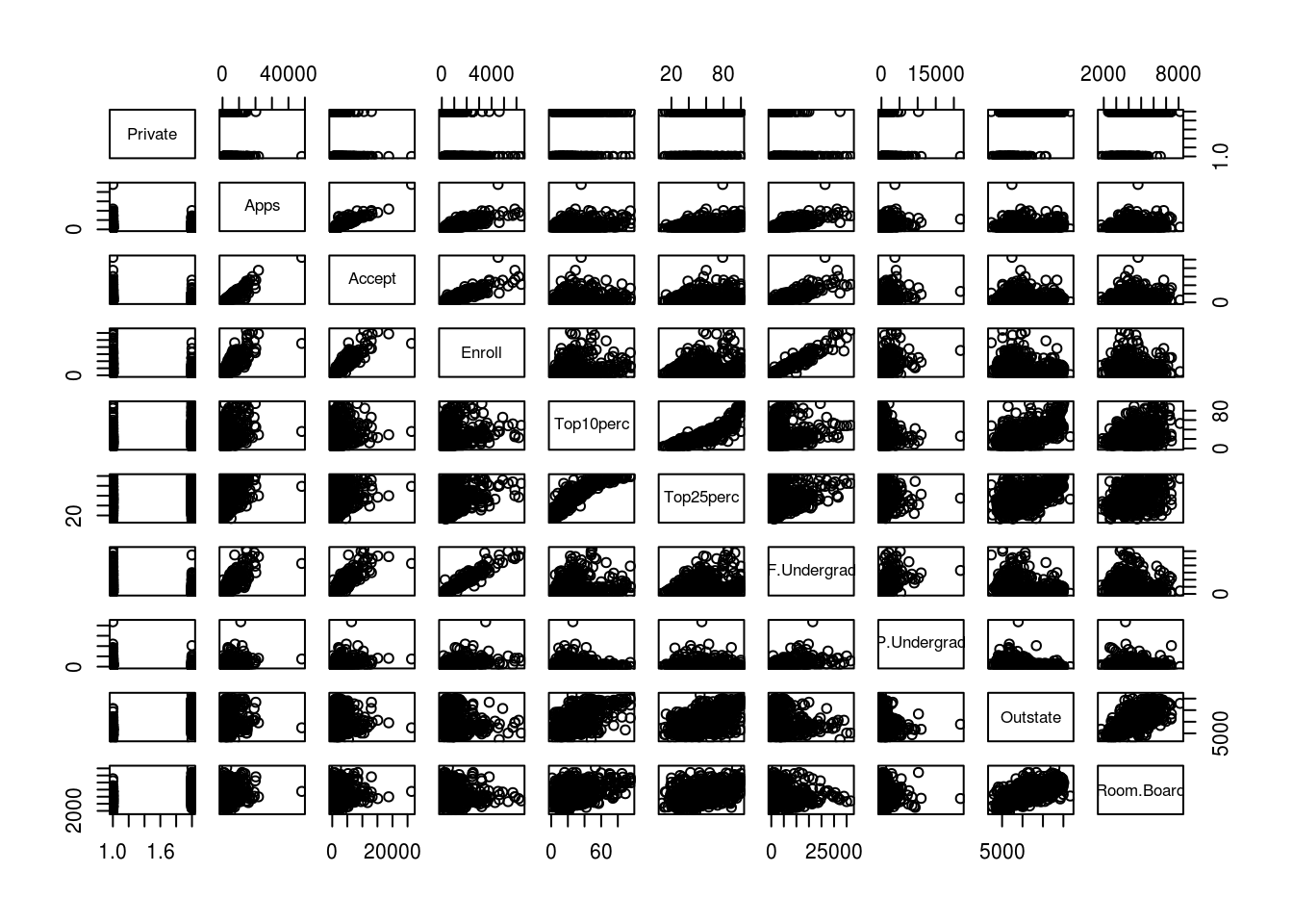
- Use the
plot()function to produce side-by-side boxplots ofOutstateversusPrivate.
plot(Outstate ~ Private, data = college,
     xlab = "Private University",
     ylab = "Tuition in $")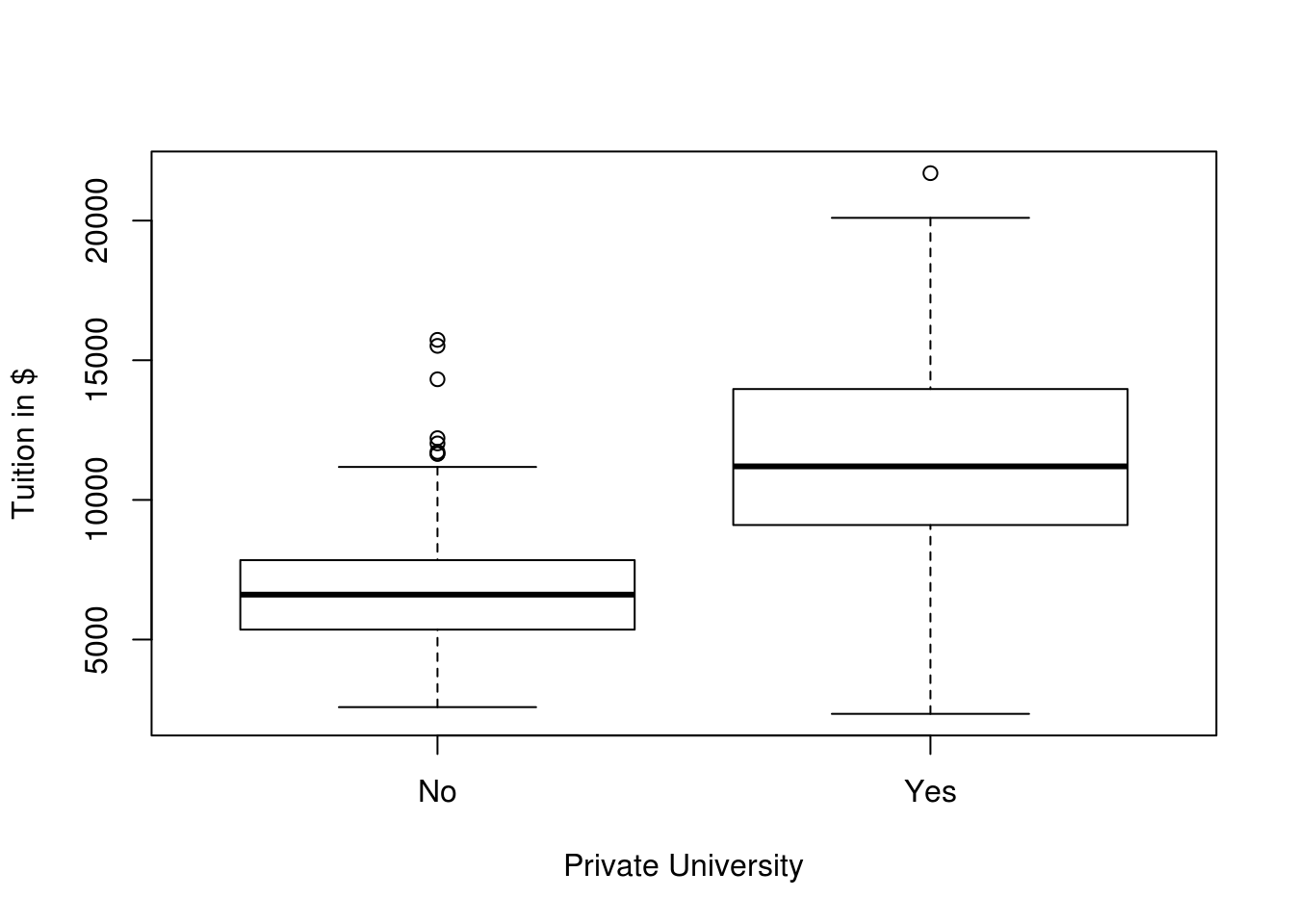
Boxplots of Outstate versus Private: Private universities have higher out of state tuition
- Create a new qualitative variable, called
Elite, by binning theTop10percvariable. We are going to divide universities into two groups based on whether or not the proportion of students coming from the top 10% of their high school classes exceeds 50%.
Elite <- rep("No", nrow(college))
Elite[college$Top10perc > 50] <- "Yes"
Elite <- as.factor(Elite)
college <- data.frame(college, Elite)
You can do the same all in one line using the ifelse function.
college$Elite <- as.factor(ifelse(college$Top10perc > 50, "Yes", "No"))Use the summary() function to see how many elite universities there are. Now use the plot() function to produce side-by-side boxplots of Outstate versus Elite.
summary(Elite) No Yes
699 78 plot(Outstate ~ Elite, data = college,
xlab = "Elite University",
ylab = "Tuition in $")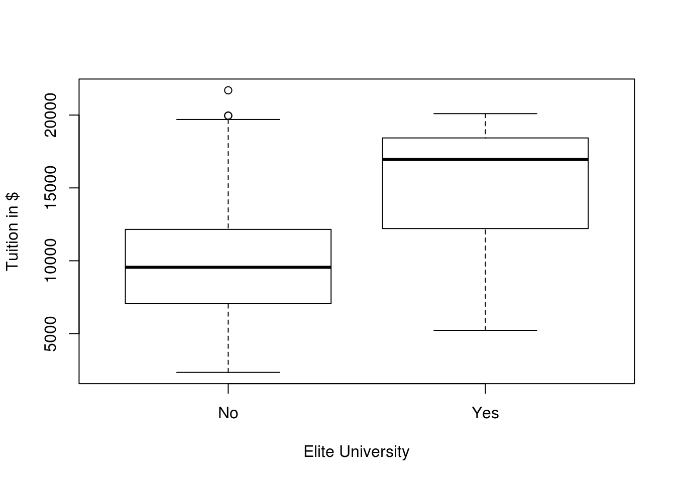
Boxplots of Outstate versus Elite: Elite universities have higher out of state tuition
- Use the
hist()function to produce some histograms with differing numbers of bins for a few of the quantitative variables. You may find the commandpar(mfrow=c(2,2))useful: it will divide the print window into four regions so that four plots can be made simultaneously. Modifying the arguments to this function will divide the screen in other ways.
par(mfrow=c(2,2))
hist(college$Apps, xlab = "Applications Received", main = "")
hist(college$perc.alumni, col=2, xlab = "% of alumni who donate", main = "")
hist(college$S.F.Ratio, col=3, breaks=10, xlab = "Student/faculty ratio", main = "")
hist(college$Expend, breaks=100, xlab = "Instructional expenditure per student", main = "")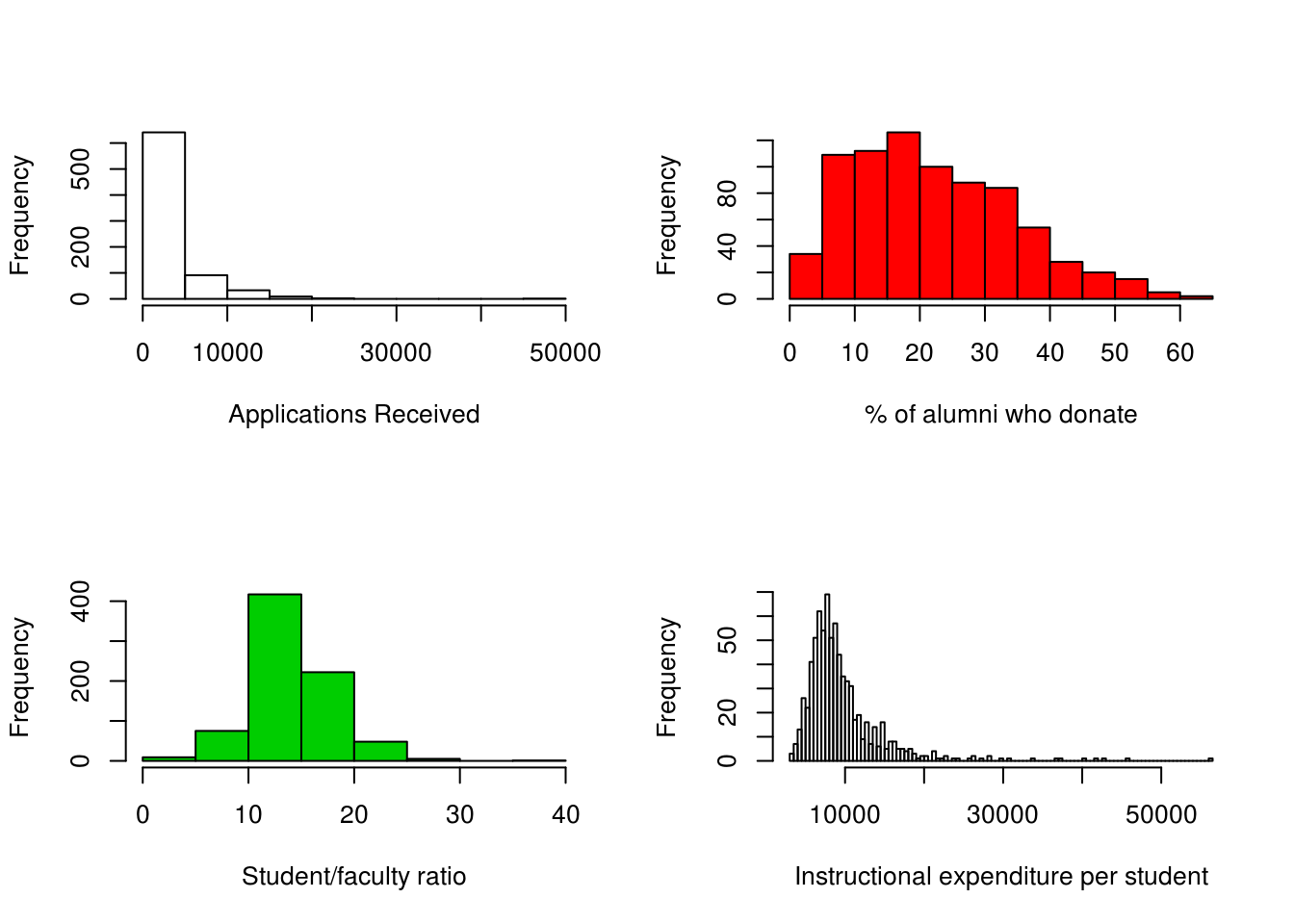
- Continue exploring the data, and provide a brief summary of what you discover.
# university with the most students in the top 10% of class
row.names(college)[which.max(college$Top10perc)]
[1] "Massachusetts Institute of Technology"acceptance_rate <- college$Accept / college$Apps
# lowest acceptance rate
row.names(college)[which.min(acceptance_rate)] [1] "Princeton University"# highest acceptance rate
row.names(college)[which.max(acceptance_rate)][1] "Emporia State University"# High tuition correlates to high graduation rate
plot(Grad.Rate ~ Outstate, data = college) 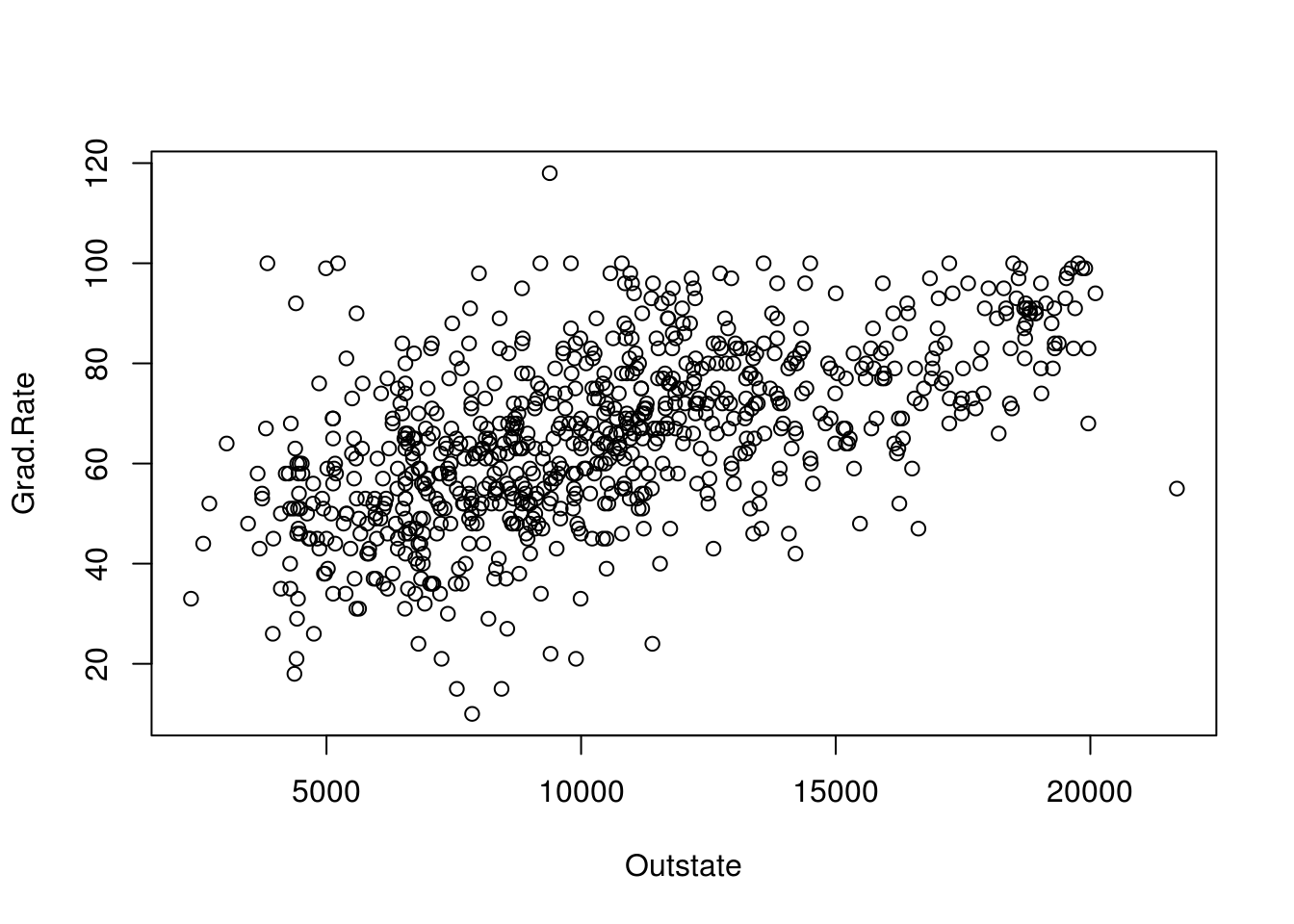
# Colleges with low acceptance rate tend to have low S:F ratio.
plot(S.F.Ratio ~ I(Accept/Apps), data = college) 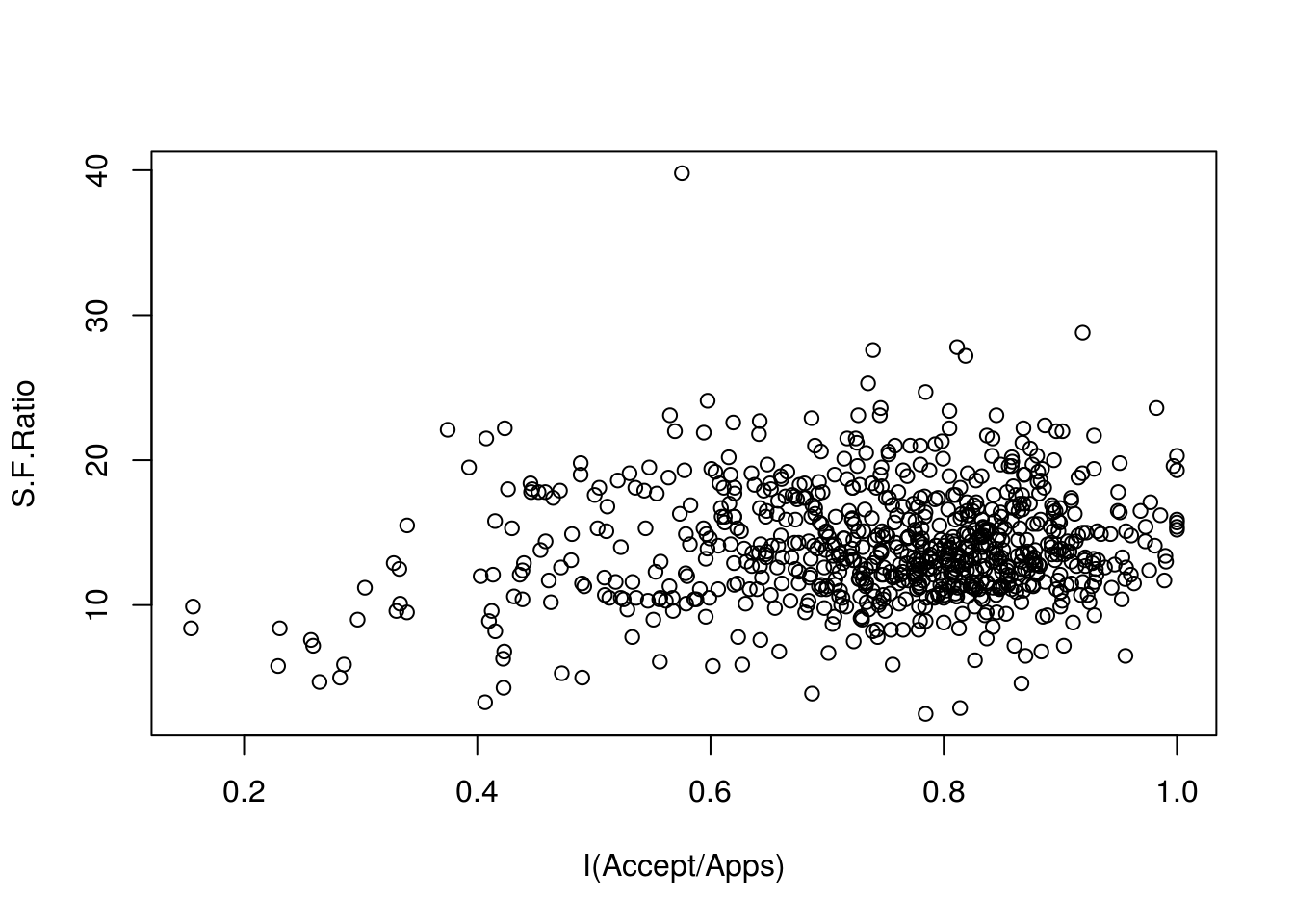
# Colleges with the most students from top 10% perc don't necessarily have
# the highest graduation rate. Also, rate > 100 is erroneous!
plot(Grad.Rate ~ Top10perc, data = college)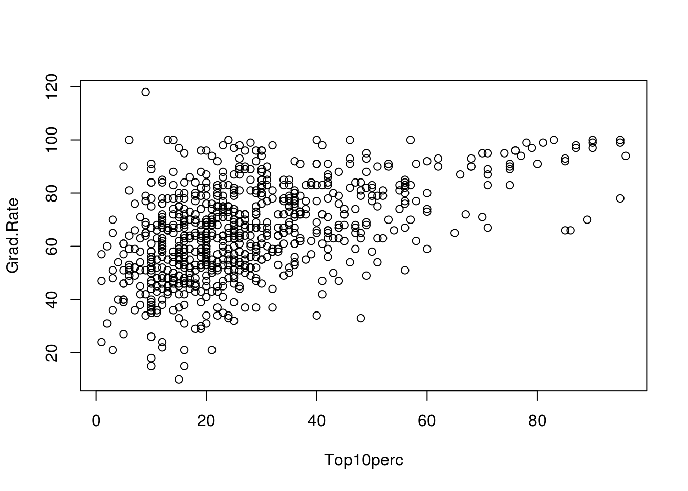
1.2.2 Exercise
This exercise involves the Auto dataset from the text book available that you can download from https://uclspp.github.io/datasets. Make sure that the missing values have been removed from the data. You should load that dataset as the first step of the exercise. Hint: We used the command for that in the Introduction to R session in class today. Go back and look up how to read in a csv file.
auto <- read.csv("Auto.csv", na.strings = "?")
auto <- na.omit(auto)
dim(auto)
[1] 392 9summary(auto) mpg cylinders displacement horsepower
Min. : 9.00 Min. :3.000 Min. : 68.0 Min. : 46.0
1st Qu.:17.00 1st Qu.:4.000 1st Qu.:105.0 1st Qu.: 75.0
Median :22.75 Median :4.000 Median :151.0 Median : 93.5
Mean :23.45 Mean :5.472 Mean :194.4 Mean :104.5
3rd Qu.:29.00 3rd Qu.:8.000 3rd Qu.:275.8 3rd Qu.:126.0
Max. :46.60 Max. :8.000 Max. :455.0 Max. :230.0
weight acceleration year origin
Min. :1613 Min. : 8.00 Min. :70.00 Min. :1.000
1st Qu.:2225 1st Qu.:13.78 1st Qu.:73.00 1st Qu.:1.000
Median :2804 Median :15.50 Median :76.00 Median :1.000
Mean :2978 Mean :15.54 Mean :75.98 Mean :1.577
3rd Qu.:3615 3rd Qu.:17.02 3rd Qu.:79.00 3rd Qu.:2.000
Max. :5140 Max. :24.80 Max. :82.00 Max. :3.000
name
amc matador : 5
ford pinto : 5
toyota corolla : 5
amc gremlin : 4
amc hornet : 4
chevrolet chevette: 4
(Other) :365 - Which of the predictors are quantitative, and which are qualitative?
Note: Sometimes when you load a dataset, a qualitative variable might have a numeric value. For instance, the origin variable is qualitative, but has integer values of 1, 2, 3. From mysterious sources (Googling), we know that this variable is coded 1 = usa; 2 = europe; 3 = japan. So we can covert it into a factor, using:
auto$originf <- factor(auto$origin, labels = c("usa", "europe", "japan"))
table(auto$originf, auto$origin)
           1   2   3
  usa    245   0   0
  europe   0  68   0
  japan    0   0  79
Quantitative: mpg, cylinders, displacement, horsepower, weight, acceleration, year.
Qualitative: name, origin, originf
- What is the range of each quantitative predictor? You can answer this using the
range()function.
#Pulling together qualitative predictors
qualitative_columns <- which(names(auto) %in% c("name", "origin", "originf"))
qualitative_columns
[1] 8 9 10# Apply the range function to the columns of auto data
# that are not qualitative
sapply(auto[, -qualitative_columns], range) mpg cylinders displacement horsepower weight acceleration year
[1,] 9.0 3 68 46 1613 8.0 70
[2,] 46.6 8 455 230 5140 24.8 82- What is the mean and standard deviation of each quantitative predictor?
sapply(auto[, -qualitative_columns], mean) mpg cylinders displacement horsepower weight
23.445918 5.471939 194.411990 104.469388 2977.584184
acceleration year
15.541327 75.979592 sapply(auto[, -qualitative_columns], sd) mpg cylinders displacement horsepower weight
7.805007 1.705783 104.644004 38.491160 849.402560
acceleration year
2.758864 3.683737 - Now remove the 10th through 85th observations. What is the range, mean, and standard deviation of each predictor in the subset of the data that remains?
sapply(auto[-seq(10, 85), -qualitative_columns], mean) mpg cylinders displacement horsepower weight
24.404430 5.373418 187.240506 100.721519 2935.971519
acceleration year
15.726899 77.145570 sapply(auto[-seq(10, 85), -qualitative_columns], sd) mpg cylinders displacement horsepower weight
7.867283 1.654179 99.678367 35.708853 811.300208
acceleration year
2.693721 3.106217 - Using the full dataset, investigate the predictors graphically, using scatterplots or other tools of your choice. Create some plots highlighting the relationships among the predictors. Comment on your findings.
pairs(auto)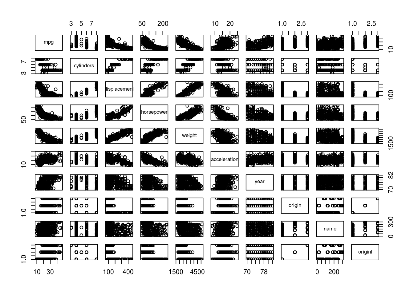
pairs(auto[, -qualitative_columns])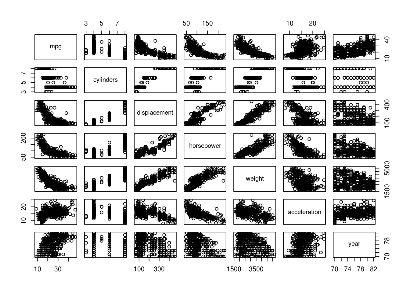
# Heavier weight correlates with lower mpg.
plot(mpg ~ weight, data = auto)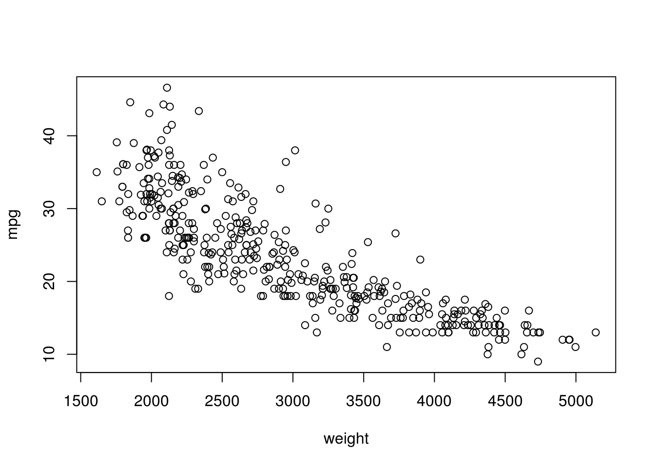
# More cylinders, less mpg.
plot(mpg ~ cylinders, data = auto)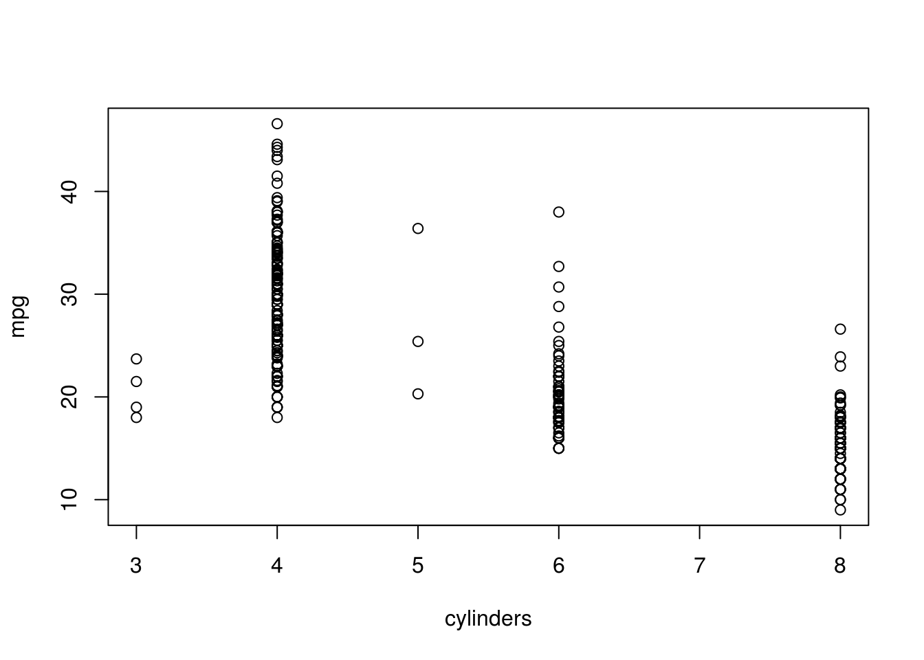
# Cars become more efficient over time.
plot(mpg ~ year, data = auto)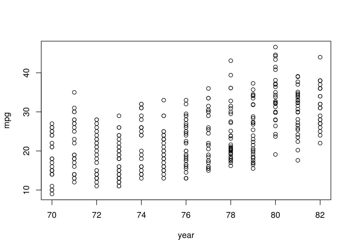
Lets plot some mpg vs. some of our qualitative features:
# sample just 20 observations
auto_sample <- auto[sample(1:nrow(auto), 20), ]

# order them
auto_sample <- auto_sample[order(auto_sample$mpg), ]

# plot them using a "dotchart"
dotchart(auto_sample$mpg, labels = auto_sample$name, xlab = "mpg")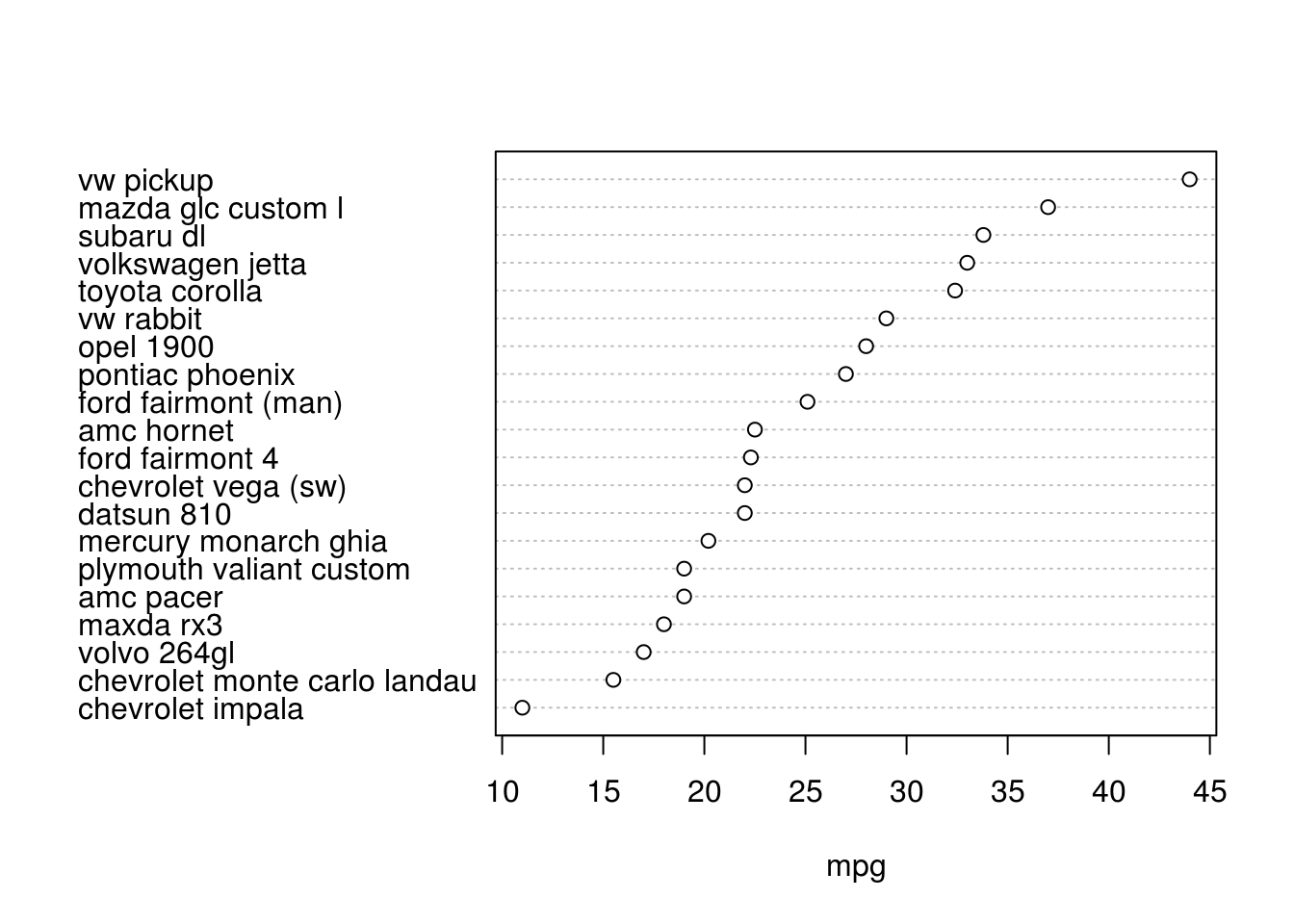
Box plot based on origin:
plot(mpg ~ originf, data = auto, ylab = "mpg")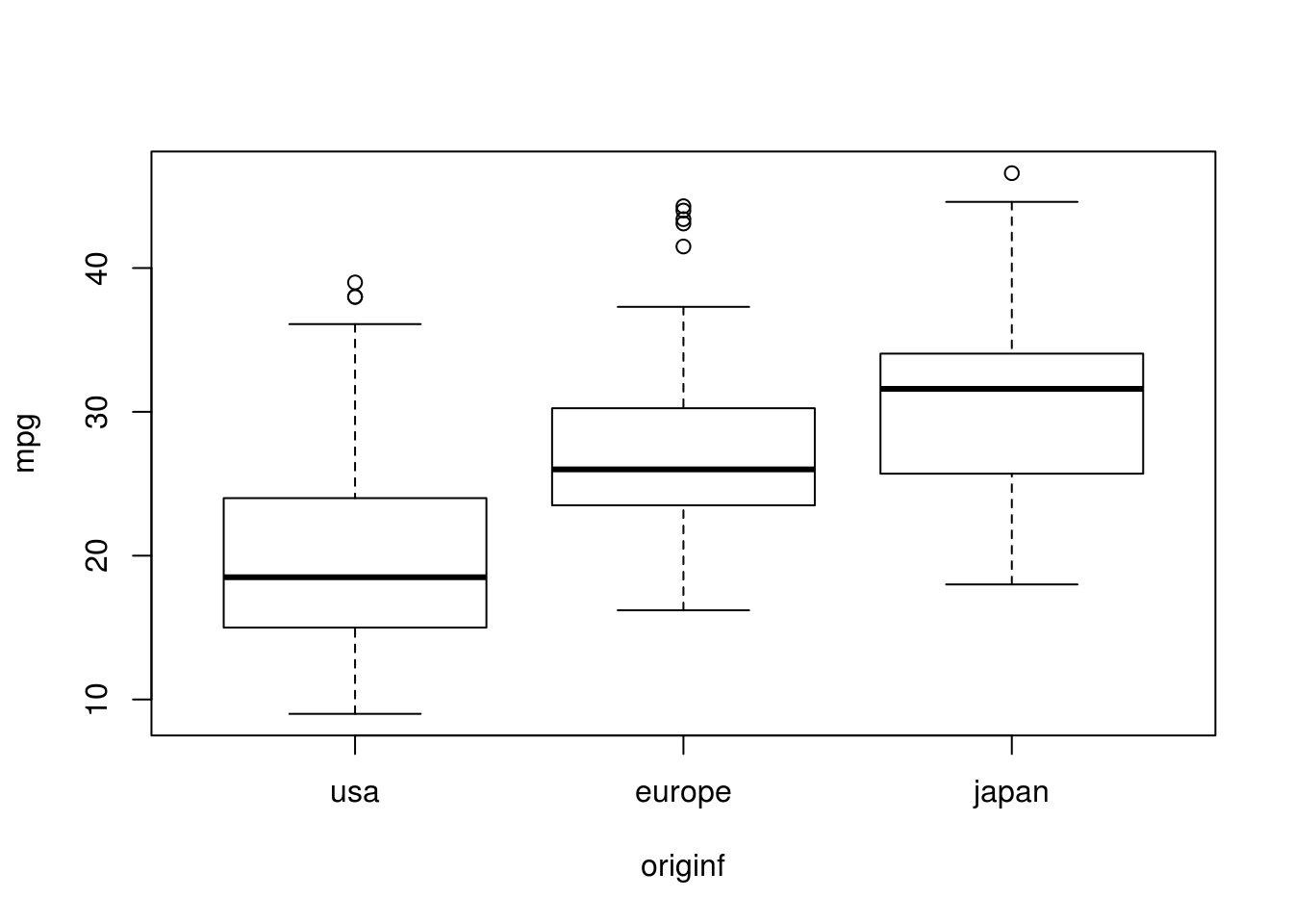
- Suppose that we wish to predict gas mileage (
mpg) on the basis of the other variables. Do your plots suggest that any of the other variables might be useful in predictingmpg? Justify your answer.
pairs(auto)
See descriptions of plots in (e). All of the predictors show some correlation with mpg. The name predictor has too little observations per name though, so using this as a predictor is likely to result in overfitting the data and will not generalize well.
1.2.3 Exercise
This exercise involves the Boston housing dataset.
- To begin, load in the
Bostondataset. TheBostondataset is part of theMASSpackage inR, and you can load by executing:
data(Boston, package = "MASS")Read about the dataset:
help(Boston, package = "MASS")How many rows are in this dataset? How many columns? What do the rows and columns represent?
dim(Boston)[1] 506 14506 rows, 14 columns. In other words: 506 housing values in Boston suburbs with 14 features each.
- Make some pairwise scatterplots of the predictors (columns) in this dataset. Describe your findings.
pairs(Boston)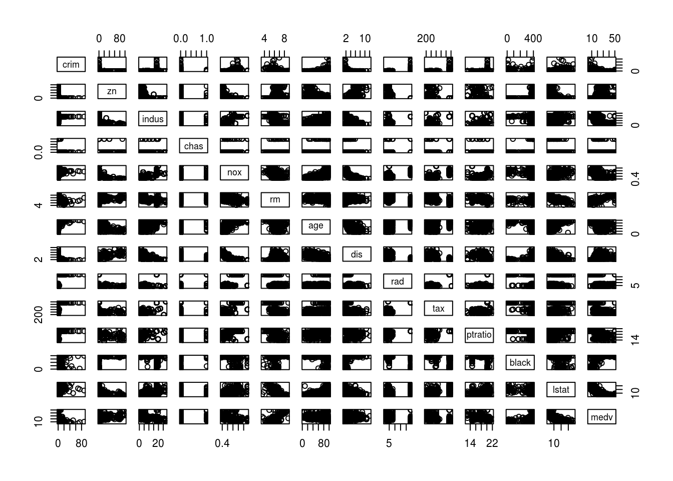
- Are any of the predictors associated with per capita crime rate? If so, explain the relationship.
plot(crim ~ age, data = Boston, log = "xy") # Older homes, more crime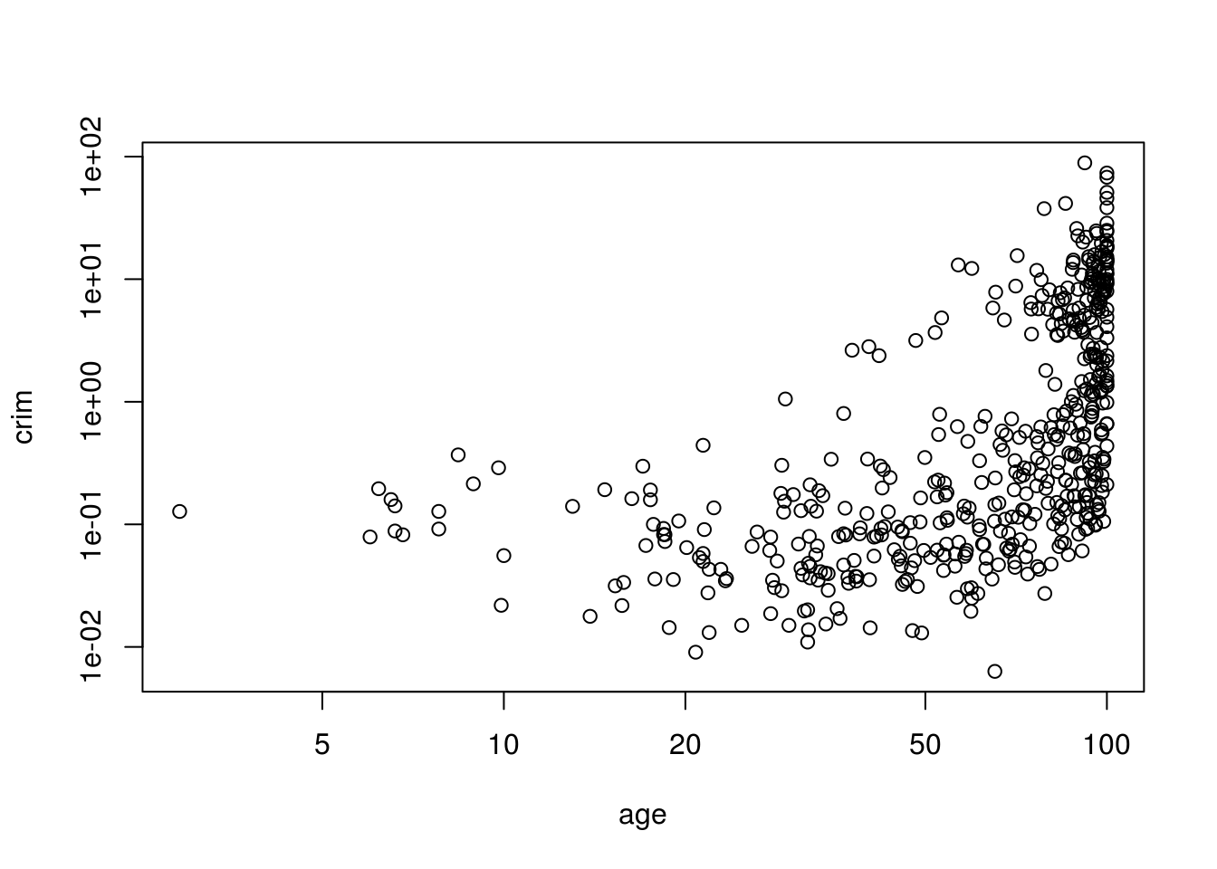
plot(crim ~ dis, data = Boston) # Closer to work-area, more crime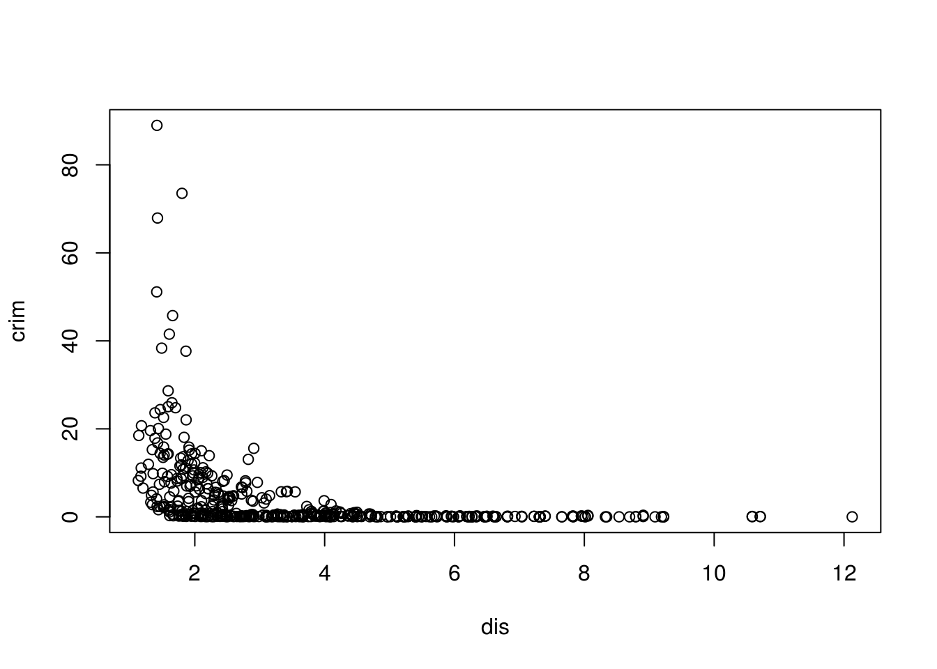
# looks much more linear with transformed on a log-log scale
plot(crim ~ dis, data = Boston, log = "xy") # Closer to work-area, more crime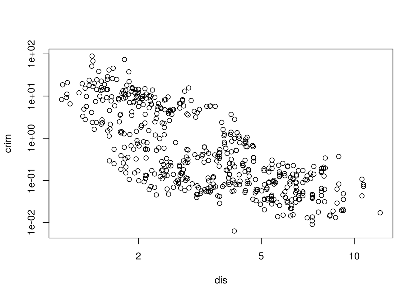
plot(crim ~ rad, data = Boston, log = "xy") # Higher index of accessibility to radial highways, more crime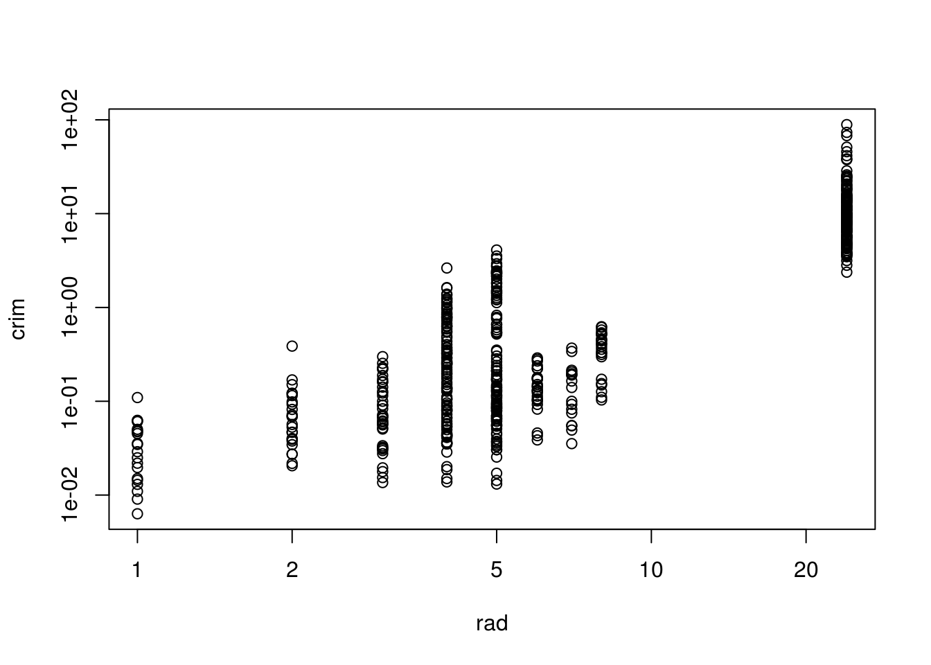
# as box plots, since rad appears to be categorical
plot(crim ~ as.factor(rad),
     log = "y",
     data = Boston,
     xlab = "Accessibility to radial highways",
     ylab = "log of crime")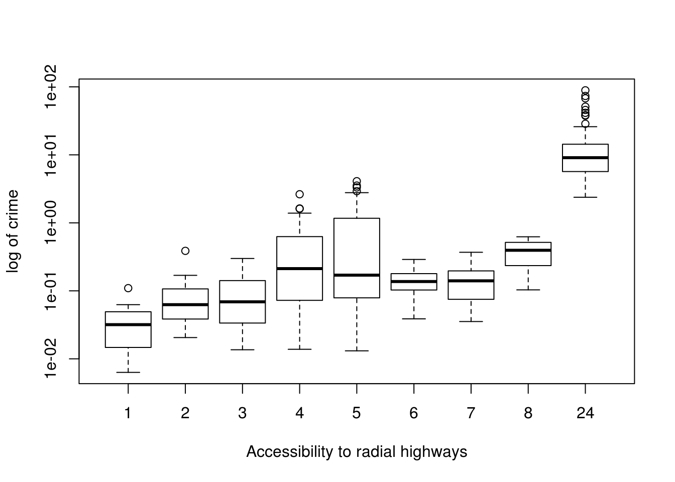
plot(crim ~ tax, log = "xy", data = Boston) # Higher tax rate, more crime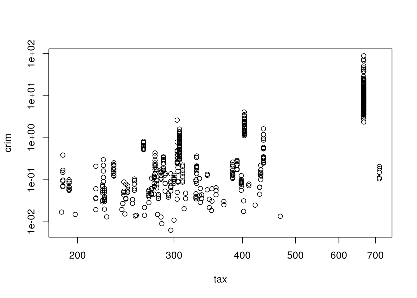
plot(crim ~ ptratio, log = "xy", data = Boston) # Higher pupil:teacher ratio, more crime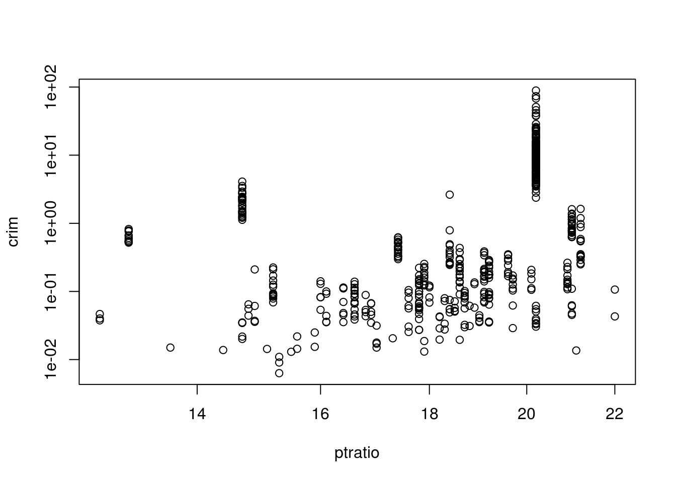
Now lets look at correlations:
cor(Boston) crim zn indus chas nox
crim 1.00000000 -0.20046922 0.40658341 -0.055891582 0.42097171
zn -0.20046922 1.00000000 -0.53382819 -0.042696719 -0.51660371
indus 0.40658341 -0.53382819 1.00000000 0.062938027 0.76365145
chas -0.05589158 -0.04269672 0.06293803 1.000000000 0.09120281
nox 0.42097171 -0.51660371 0.76365145 0.091202807 1.00000000
rm -0.21924670 0.31199059 -0.39167585 0.091251225 -0.30218819
age 0.35273425 -0.56953734 0.64477851 0.086517774 0.73147010
dis -0.37967009 0.66440822 -0.70802699 -0.099175780 -0.76923011
rad 0.62550515 -0.31194783 0.59512927 -0.007368241 0.61144056
tax 0.58276431 -0.31456332 0.72076018 -0.035586518 0.66802320
ptratio 0.28994558 -0.39167855 0.38324756 -0.121515174 0.18893268
black -0.38506394 0.17552032 -0.35697654 0.048788485 -0.38005064
lstat 0.45562148 -0.41299457 0.60379972 -0.053929298 0.59087892
medv -0.38830461 0.36044534 -0.48372516 0.175260177 -0.42732077
rm age dis rad tax
crim -0.21924670 0.35273425 -0.37967009 0.625505145 0.58276431
zn 0.31199059 -0.56953734 0.66440822 -0.311947826 -0.31456332
indus -0.39167585 0.64477851 -0.70802699 0.595129275 0.72076018
chas 0.09125123 0.08651777 -0.09917578 -0.007368241 -0.03558652
nox -0.30218819 0.73147010 -0.76923011 0.611440563 0.66802320
rm 1.00000000 -0.24026493 0.20524621 -0.209846668 -0.29204783
age -0.24026493 1.00000000 -0.74788054 0.456022452 0.50645559
dis 0.20524621 -0.74788054 1.00000000 -0.494587930 -0.53443158
rad -0.20984667 0.45602245 -0.49458793 1.000000000 0.91022819
tax -0.29204783 0.50645559 -0.53443158 0.910228189 1.00000000
ptratio -0.35550149 0.26151501 -0.23247054 0.464741179 0.46085304
black 0.12806864 -0.27353398 0.29151167 -0.444412816 -0.44180801
lstat -0.61380827 0.60233853 -0.49699583 0.488676335 0.54399341
medv 0.69535995 -0.37695457 0.24992873 -0.381626231 -0.46853593
ptratio black lstat medv
crim 0.2899456 -0.38506394 0.4556215 -0.3883046
zn -0.3916785 0.17552032 -0.4129946 0.3604453
indus 0.3832476 -0.35697654 0.6037997 -0.4837252
chas -0.1215152 0.04878848 -0.0539293 0.1752602
nox 0.1889327 -0.38005064 0.5908789 -0.4273208
rm -0.3555015 0.12806864 -0.6138083 0.6953599
age 0.2615150 -0.27353398 0.6023385 -0.3769546
dis -0.2324705 0.29151167 -0.4969958 0.2499287
rad 0.4647412 -0.44441282 0.4886763 -0.3816262
tax 0.4608530 -0.44180801 0.5439934 -0.4685359
ptratio 1.0000000 -0.17738330 0.3740443 -0.5077867
black -0.1773833 1.00000000 -0.3660869 0.3334608
lstat 0.3740443 -0.36608690 1.0000000 -0.7376627
medv -0.5077867 0.33346082 -0.7376627 1.0000000- Do any of the suburbs of Boston appear to have particularly high crime rates? Tax rates? Pupil-teacher ratios? Comment on the range of each predictor.
par(mfrow=c(1,3))
hist(Boston$crim[Boston$crim > 1], breaks=25)
# most cities have low crime rates, but there is a long tail: 18 suburbs appear
# to have a crime rate > 20, reaching to above 80

hist(Boston$tax, breaks=25)
# there is a large divide between suburbs with low tax rates and a peak at 660-680

hist(Boston$ptratio, breaks=25)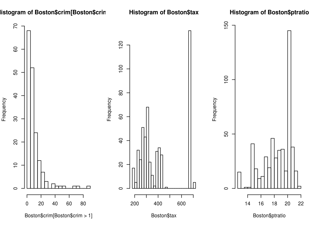
# a skew towards high ratios, but no particularly high ratios- How many of the suburbs in this dataset bound the Charles river?
sum(Boston$chas == 1)[1] 3535
- What is the median pupil-teacher ratio among the towns in this dataset?
median(Boston$ptratio)[1] 19.0519.05
- Which suburb of Boston has lowest median value of owner-occupied homes? What are the values of the other predictors for that suburb, and how do those values compare to the overall ranges for those predictors? Comment on your findings.
t(subset(Boston, medv == min(medv))) 399 406
crim 38.3518 67.9208
zn 0.0000 0.0000
indus 18.1000 18.1000
chas 0.0000 0.0000
nox 0.6930 0.6930
rm 5.4530 5.6830
age 100.0000 100.0000
dis 1.4896 1.4254
rad 24.0000 24.0000
tax 666.0000 666.0000
ptratio 20.2000 20.2000
black 396.9000 384.9700
lstat 30.5900 22.9800
medv 5.0000 5.0000# 399 406
# crim 38.3518 67.9208 above 3rd quartile
# zn 0.0000 0.0000 at min
# indus 18.1000 18.1000 at 3rd quartile
# chas 0.0000 0.0000 not bounded by river
# nox 0.6930 0.6930 above 3rd quartile
# rm 5.4530 5.6830 below 1st quartile
# age 100.0000 100.0000 at max
# dis 1.4896 1.4254 below 1st quartile
# rad 24.0000 24.0000 at max
# tax 666.0000 666.0000 at 3rd quartile
# ptratio 20.2000 20.2000 at 3rd quartile
# black 396.9000 384.9700 at max; above 1st quartile
# lstat 30.5900 22.9800 above 3rd quartile
# medv 5.0000 5.0000 at minNow lets print out a summary:
summary(Boston) crim zn indus chas
Min. : 0.00632 Min. : 0.00 Min. : 0.46 Min. :0.00000
1st Qu.: 0.08204 1st Qu.: 0.00 1st Qu.: 5.19 1st Qu.:0.00000
Median : 0.25651 Median : 0.00 Median : 9.69 Median :0.00000
Mean : 3.61352 Mean : 11.36 Mean :11.14 Mean :0.06917
3rd Qu.: 3.67708 3rd Qu.: 12.50 3rd Qu.:18.10 3rd Qu.:0.00000
Max. :88.97620 Max. :100.00 Max. :27.74 Max. :1.00000
nox rm age dis
Min. :0.3850 Min. :3.561 Min. : 2.90 Min. : 1.130
1st Qu.:0.4490 1st Qu.:5.886 1st Qu.: 45.02 1st Qu.: 2.100
Median :0.5380 Median :6.208 Median : 77.50 Median : 3.207
Mean :0.5547 Mean :6.285 Mean : 68.57 Mean : 3.795
3rd Qu.:0.6240 3rd Qu.:6.623 3rd Qu.: 94.08 3rd Qu.: 5.188
Max. :0.8710 Max. :8.780 Max. :100.00 Max. :12.127
rad tax ptratio black
Min. : 1.000 Min. :187.0 Min. :12.60 Min. : 0.32
1st Qu.: 4.000 1st Qu.:279.0 1st Qu.:17.40 1st Qu.:375.38
Median : 5.000 Median :330.0 Median :19.05 Median :391.44
Mean : 9.549 Mean :408.2 Mean :18.46 Mean :356.67
3rd Qu.:24.000 3rd Qu.:666.0 3rd Qu.:20.20 3rd Qu.:396.23
Max. :24.000 Max. :711.0 Max. :22.00 Max. :396.90
lstat medv
Min. : 1.73 Min. : 5.00
1st Qu.: 6.95 1st Qu.:17.02
Median :11.36 Median :21.20
Mean :12.65 Mean :22.53
3rd Qu.:16.95 3rd Qu.:25.00
Max. :37.97 Max. :50.00 - In this dataset, how many of the suburbs average more than seven rooms per dwelling? More than eight rooms per dwelling? Comment on the suburbs that average more than eight rooms per dwelling.
sum(Boston$rm > 7)[1] 64sum(Boston$rm > 8)[1] 13Suburbs that average more than eight rooms per dwelling:
summary(subset(Boston, rm > 8)) crim zn indus chas
Min. :0.02009 Min. : 0.00 Min. : 2.680 Min. :0.0000
1st Qu.:0.33147 1st Qu.: 0.00 1st Qu.: 3.970 1st Qu.:0.0000
Median :0.52014 Median : 0.00 Median : 6.200 Median :0.0000
Mean :0.71879 Mean :13.62 Mean : 7.078 Mean :0.1538
3rd Qu.:0.57834 3rd Qu.:20.00 3rd Qu.: 6.200 3rd Qu.:0.0000
Max. :3.47428 Max. :95.00 Max. :19.580 Max. :1.0000
nox rm age dis
Min. :0.4161 Min. :8.034 Min. : 8.40 Min. :1.801
1st Qu.:0.5040 1st Qu.:8.247 1st Qu.:70.40 1st Qu.:2.288
Median :0.5070 Median :8.297 Median :78.30 Median :2.894
Mean :0.5392 Mean :8.349 Mean :71.54 Mean :3.430
3rd Qu.:0.6050 3rd Qu.:8.398 3rd Qu.:86.50 3rd Qu.:3.652
Max. :0.7180 Max. :8.780 Max. :93.90 Max. :8.907
rad tax ptratio black
Min. : 2.000 Min. :224.0 Min. :13.00 Min. :354.6
1st Qu.: 5.000 1st Qu.:264.0 1st Qu.:14.70 1st Qu.:384.5
Median : 7.000 Median :307.0 Median :17.40 Median :386.9
Mean : 7.462 Mean :325.1 Mean :16.36 Mean :385.2
3rd Qu.: 8.000 3rd Qu.:307.0 3rd Qu.:17.40 3rd Qu.:389.7
Max. :24.000 Max. :666.0 Max. :20.20 Max. :396.9
lstat medv
Min. :2.47 Min. :21.9
1st Qu.:3.32 1st Qu.:41.7
Median :4.14 Median :48.3
Mean :4.31 Mean :44.2
3rd Qu.:5.12 3rd Qu.:50.0
Max. :7.44 Max. :50.0 summary(Boston) crim zn indus chas
Min. : 0.00632 Min. : 0.00 Min. : 0.46 Min. :0.00000
1st Qu.: 0.08204 1st Qu.: 0.00 1st Qu.: 5.19 1st Qu.:0.00000
Median : 0.25651 Median : 0.00 Median : 9.69 Median :0.00000
Mean : 3.61352 Mean : 11.36 Mean :11.14 Mean :0.06917
3rd Qu.: 3.67708 3rd Qu.: 12.50 3rd Qu.:18.10 3rd Qu.:0.00000
Max. :88.97620 Max. :100.00 Max. :27.74 Max. :1.00000
nox rm age dis
Min. :0.3850 Min. :3.561 Min. : 2.90 Min. : 1.130
1st Qu.:0.4490 1st Qu.:5.886 1st Qu.: 45.02 1st Qu.: 2.100
Median :0.5380 Median :6.208 Median : 77.50 Median : 3.207
Mean :0.5547 Mean :6.285 Mean : 68.57 Mean : 3.795
3rd Qu.:0.6240 3rd Qu.:6.623 3rd Qu.: 94.08 3rd Qu.: 5.188
Max. :0.8710 Max. :8.780 Max. :100.00 Max. :12.127
rad tax ptratio black
Min. : 1.000 Min. :187.0 Min. :12.60 Min. : 0.32
1st Qu.: 4.000 1st Qu.:279.0 1st Qu.:17.40 1st Qu.:375.38
Median : 5.000 Median :330.0 Median :19.05 Median :391.44
Mean : 9.549 Mean :408.2 Mean :18.46 Mean :356.67
3rd Qu.:24.000 3rd Qu.:666.0 3rd Qu.:20.20 3rd Qu.:396.23
Max. :24.000 Max. :711.0 Max. :22.00 Max. :396.90
lstat medv
Min. : 1.73 Min. : 5.00
1st Qu.: 6.95 1st Qu.:17.02
Median :11.36 Median :21.20
Mean :12.65 Mean :22.53
3rd Qu.:16.95 3rd Qu.:25.00
Max. :37.97 Max. :50.00 Relatively lower crime (comparing range), lower lstat (comparing range)