Text Analysis

Wordscores

library(countrycode)
library(classInt)
library(tidyverse)
library(maps)
library(rworldmap)
library(quanteda)
library(readtext)
library(RColorBrewer)

Load the UNGD data. Make sure you’ve downloaded the dataset from http://dx.doi.org/10.7910/DVN/0TJX8Y and placed it in your working directory.

ungd_debates <- readtext("UNGDC 1970-2016.zip",
                         ignore_missing_files = TRUE,
                         docvarsfrom = "filenames",
                         dvsep = "_",
                         docvarnames = c("country", "session", "year"),
                         verbosity = 0)

Create a corpus from the texts.

ungd_corpus <- corpus(ungd_debates)

Create a subset that only includes debates from 2014. We focus on 2014 to analyse the idealogical positions of countries during the crisis in Ukraine.

ungd_2014 <- corpus_subset(ungd_corpus, year == 2014)

Save the docvars in a data.frame that we’ll use later.

ungd_data <- as.data.frame(docvars(ungd_2014))

Create a document-feature matrix.

ungd_dfm <- dfm(ungd_2014,
                stem = TRUE,
                remove = stopwords("english"),
                remove_punct = TRUE,
                remove_numbers = TRUE)

ungd_dfm <- dfm_trim(ungd_dfm, min_count = 10, min_docfreq = 5)

Assuming that U.S. and Russia represent the two extremes of idealogical positions over the Ukrainian crisis, we set the the reference scores as follows:

RUS = -1
USA = 1

First, we find the index of RUS and USA debates.

rus_index <- which(ungd_data$country == "RUS")
usa_index <- which(ungd_data$country == "USA")

Then we set the reference scrores for RUS and USA and leave the rest to NA.

refscores <- rep(NA, nrow(ungd_dfm))
refscores[rus_index] <- -1
refscores[usa_index] <- 1

Fit a wordscores model using the reference scores.

wordscores_model <- textmodel(ungd_dfm,
                              refscores,
                              model = "wordscores",
                              scale = "linear",
                              smooth = 1)

Extract the wordscores, rescale them and then save in ungd_data data.frame we created earlier.

wordscores <- predict(wordscores_model, rescaling = "mv")

ungd_data$wordscore <- wordscores@textscores$textscore_mv

You can use the wordscore estimates as explanatory variables to understand how the policy dimension affects some other response variable that you’re interested in.

Let’s see what the ungd_data looks like:

head(ungd_data)

                                    doc_id country session year  wordscore
text7121 Session 69 - 2014/AFG_69_2014.txt     AFG      69 2014 -0.3351900
text7122 Session 69 - 2014/AGO_69_2014.txt     AGO      69 2014 -0.4436961
text7123 Session 69 - 2014/ALB_69_2014.txt     ALB      69 2014 -0.3489190
text7124 Session 69 - 2014/AND_69_2014.txt     AND      69 2014 -0.1707580
text7125 Session 69 - 2014/ARE_69_2014.txt     ARE      69 2014 -0.2457200
text7126 Session 69 - 2014/ARG_69_2014.txt     ARG      69 2014 -0.2114322

Use classIntervals to create breaks between the continous scale from -1 to 1. We’ll need this for plotting.

class_intervals <- classIntervals(ungd_data$wordscore, 
                                  rtimes = 10,
                                  style = 'bclust')

Committee Member: 1(1) 2(1) 3(1) 4(1) 5(1) 6(1) 7(1) 8(1) 9(1) 10(1)
Computing Hierarchical Clustering

Plotting with rworldmap

You can use rworldmap package for plotting.

spatial_data <- joinCountryData2Map(ungd_data,
                                    joinCode = "ISO3", 
                                    nameJoinColumn = "country")

192 codes from your data successfully matched countries in the map
2 codes from your data failed to match with a country code in the map
51 codes from the map weren't represented in your data

wordscore_map <- mapCountryData(spatial_data,
                                nameColumnToPlot = "wordscore",
                                catMethod = class_intervals$brks,
                                mapTitle = "Russia vs USA: Wordscores 2014",
                                colourPalette = brewer.pal(9, "Blues"),
                                missingCountryCol = "grey",
                                addLegend = FALSE)

do.call(addMapLegend, c(wordscore_map, 
                        legendLabels = "limits",
                        labelFontSize = 0.7,
                        legendShrink = 0.7,
                        legendMar = 5, 
                        legendWidth = 0.5))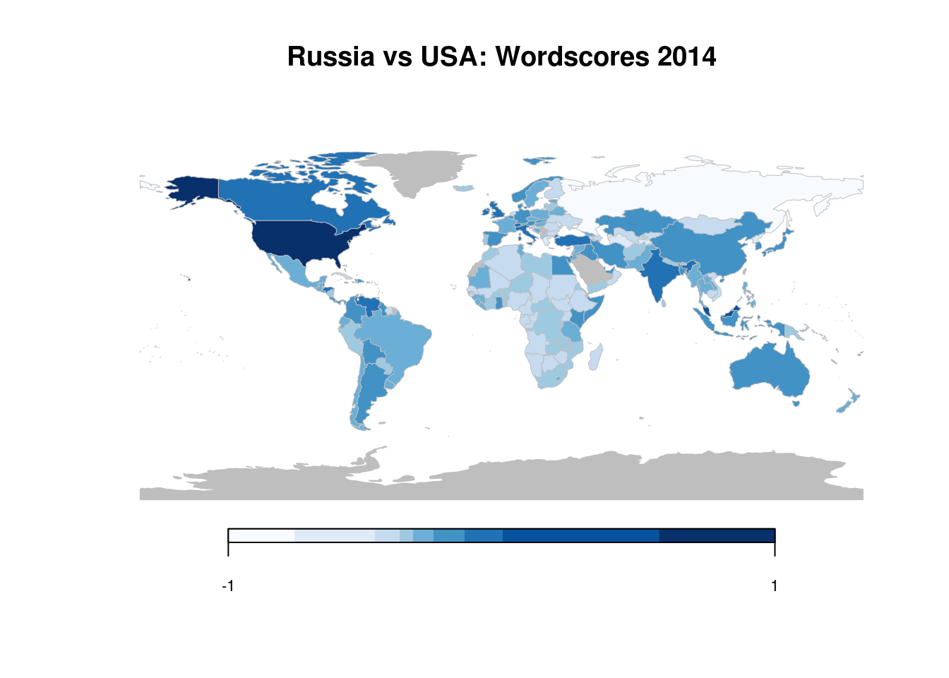

Plotting with ggplot

ungd_data$wordscore_int <- cut(ungd_data$wordscore, 
                               include.lowest = TRUE,
                               breaks = class_intervals$brks)

Merge map data with wordscores for plotting.

world_map <- map_data("world")

world_map$country <- countrycode(world_map$region, 
                                 "country.name", 
                                 "iso3c")

Warning in countrycode(world_map$region, "country.name", "iso3c"): Some values were not matched unambiguously: Ascension Island, Azores, Barbuda, Bonaire, Canary Islands, Chagos Archipelago, Grenadines, Heard Island, Kosovo, Madeira Islands, Micronesia, Saba, Saint Martin, Siachen Glacier, Sint Eustatius, Virgin Islands

world_map <- inner_join(world_map, 
                        ungd_data,
                        by = c("country"))

world_map <- subset(world_map, select = c(lat, long, group, wordscore_int))

Create the plot and customize the appearance.

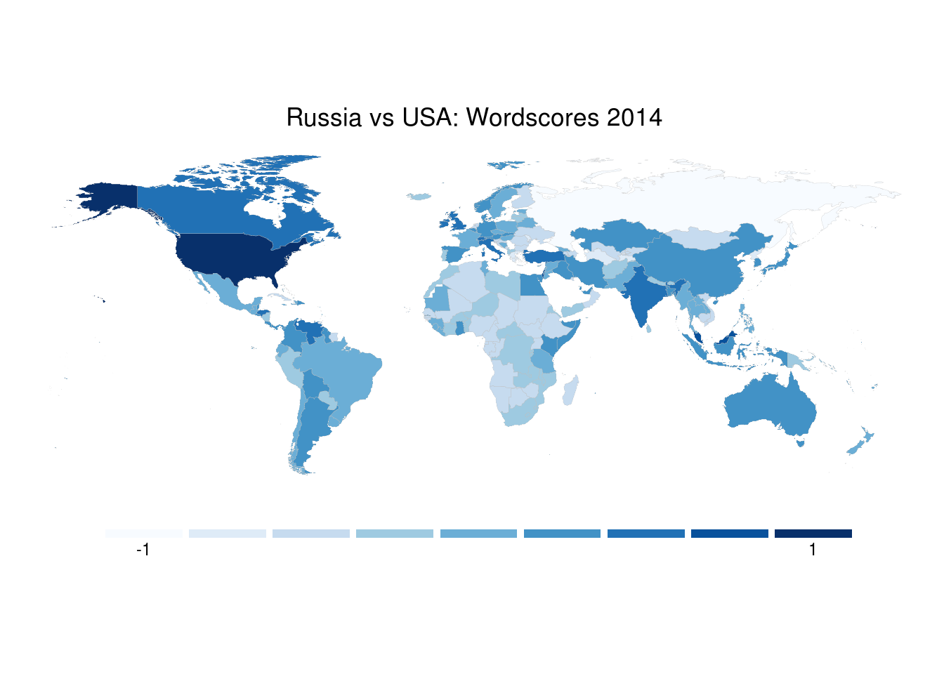
ggplot(world_map, aes(long, lat, group = group)) +
  ggtitle("Russia vs USA: Wordscores 2014") +
  geom_polygon(aes(fill = wordscore_int)) +
  geom_path(color = "grey", size = 0.05) +
  scale_fill_brewer(
    palette = "Blues", 
    labels = c(-1, rep("", 7), 1),
    guide = guide_legend(
      nrow = 1, 
      label.hjust = 0.5, 
      label.position = "bottom"
    )
  ) +
  coord_equal() +
  theme_void() +
  theme(
    plot.title = element_text(hjust = 0.5),
    legend.title = element_blank(),
    legend.position = "bottom",
    legend.direction = "horizontal",
    legend.key.width = unit(15, units = "mm"),
    legend.key.height = unit(2, units = "mm")
  )